Demonstration using symmetrized harmonics

This notebook demonstrates the reconstruction workflow for a single-slice reconstruction using symmetrized spherical harmonics. The harmonics workflow is faster than the RBF workflow but usually give worse results.

1. Imports

import matplotlib.pyplot as plt
import matplotlib.gridspec as gridspec
import numpy as np
from odftomo import plot_tools

from odftomo.io import load_series, slice_geometry
from odftomo.tomography_models import FromArrayModel
from odftomo.optimization import FISTA

from odftomo.texture import odfs, point_groups
from odftomo.spharm.symmetrized_harmonics_coefficients import make_symmetrized_harmonics
from odftomo.crystallography import cubic
from odftomo.spharm import map_from_spharm_coefficients, GSH_mapper
from odftomo.spharm.spharm_tools import map_single_l

import logging
logger = logging.getLogger()
logger.setLevel(logging.ERROR)

INFO:Setting the number of threads to 8. If your physical cores are fewer than this number, you may want to use numba.set_num_threads(n), and os.environ["OPENBLAS_NUM_THREADS"] = f"{n}" to set the number of threads to the number of physical cores n.
INFO:Setting numba log level to WARNING.

2. Loading data

We use the mumott data loader to ensure compatibility. Because mumott does for now not have explicit support for files with multiple q-bins, this involves separately loading a file for each q-bin. odftomo.io.load_series wraps this behaviour and outputs the arrays we need:

1. data_array is a 5D numpy array containing the azimtuthally regrouped data ordered like: 0 sample rotation, 1 first raster scan index, 2 second raster scan index ( for a single-slice experiment this should have length 1), 3 detector azimuthal angle, 4 bragg peak number.

2. weigth_array used to weight the residual for optimization. Mainly used to mask out bad data. Same shape as data_array.

3. coordinates unit vectors of the q-space direction in sample-fixed coordinates probed by each data point. The shape of the array shoudl match data_array but with one-length dimensions for the two raster-scan indexes: Shape is 0 sample rotation, 1 and 2 are 1-length dimensions corresponding the the sample-scannign directions used to make broadcasting easier, the 3 index is the detector azimuth, 4 bragg peak number and 5 is the vector xyz index.

4. geometry mumott geometry object used to initialize the projector object later which is used to calculate radon transforms. For a description of this object see mumott.org.

The data used for this demonstration is publically available at: https://zenodo.org/records/10889439

wget https://zenodo.org/records/10889439/files/gamma_111.h5 https://zenodo.org/records/10889439/files/gamma_200.h5 https://zenodo.org/records/10889439/files/gamma_220.h5

hkl_list = [(1, 1, 1),
            (2, 0, 0),
            (2, 2, 0),]
files = [f'gamma_{h[0]}{h[1]}{h[2]}.h5' for h in hkl_list]
data_array, weigth_array, coordinates, full_geom = load_series(files)

/das/home/carlse_m/mumott_dev_version/mumott/mumott/data_handling/data_container.py:227: DeprecationWarning: Entry name rotations is deprecated. Use inner_angle instead.
  _deprecated_key_warning('rotations')
/das/home/carlse_m/mumott_dev_version/mumott/mumott/data_handling/data_container.py:236: DeprecationWarning: Entry name tilts is deprecated. Use outer_angle instead.
  _deprecated_key_warning('tilts')
/das/home/carlse_m/mumott_dev_version/mumott/mumott/data_handling/data_container.py:268: DeprecationWarning: Entry name offset_j is deprecated. Use j_offset instead.
  _deprecated_key_warning('offset_j')
/das/home/carlse_m/mumott_dev_version/mumott/mumott/data_handling/data_container.py:278: DeprecationWarning: Entry name offset_k is deprecated. Use k_offset instead.
  _deprecated_key_warning('offset_k')
/das/home/carlse_m/grids_in_so3/odftt/io/mumott_fileformat_loader.py:26: RuntimeWarning: invalid value encountered in divide
  data_arrays.append(np.array(data_container.data / data_container.diode[:, :, :, np.newaxis]))

For this demonstration to run quickly on slow hardware, we reconstruct only a 2D slice. This block can be omitted if you want to do a 3D reconstruction, but it will be slow! We achieve a 2D geometry by removing all measurements with tilt-angle not equal to 0 and to select only a single 1D slice of the 2D raster scans.

# Include only projecitons with zero tilt.
data_array = data_array[:50, ...]
weigth_array = weigth_array[:50, ...]
coordinates = coordinates[:50, ...]
geom = slice_geometry(full_geom, slice(50))

# Crop out a single 1D slice of the 2D raster scans
data_slice = data_array[:,:,25:26,:,:]
weigth_slice = weigth_array[:,:,25:26,:,:]

# Make a new mumott geometry object corresponding to the 2D geometry
from mumott.core.geometry import Geometry, GeometryTuple
geom_slice = Geometry()
for gt in geom:
    gt_new = GeometryTuple(rotation = gt.rotation, k_offset = 0.0, j_offset = 0)
    geom_slice.append(gt_new)
geom_slice.volume_shape = np.array([60, 1, 60])
geom_slice.projection_shape = np.array([54, 1])
geom_slice.p_direction_0 = geom.p_direction_0
geom_slice.j_direction_0 = geom.j_direction_0
geom_slice.k_direction_0 = geom.k_direction_0
geom_slice.detector_direction_origin = geom.detector_direction_origin
geom_slice.detector_direction_positive_90 = geom.detector_direction_positive_90
geom_slice.detector_angles = geom.detector_angles
geom_slice.full_circle_covered = geom.full_circle_covered

The data in these files has not yet been normalized by the scaling-factors. We estimate the scaling factors form the data and normalize it out of the data.

data_array[np.isnan(data_array) ] = 0
data_array[np.isinf(data_array) ] = 0
solidangle_factor = np.abs(np.cos(geom_slice.detector_angles))[np.newaxis,np.newaxis,np.newaxis,:,np.newaxis] * np.ones(data_array.shape)
intensity_scaling_factors = np.mean(data_array * solidangle_factor, axis = (0,1,2,3)) / np.mean(solidangle_factor, axis = (0,1,2,3))
intensity_scaling_factors = intensity_scaling_factors/intensity_scaling_factors[0]
data_slice = data_slice / intensity_scaling_factors[np.newaxis, np.newaxis, np.newaxis, np.newaxis, :]

3. Define reconstruction model

The odf object abstractly represents a model for an ODF and calculates the probablity density, pole-figures and inverse pole figures of each basis function.

In this demonstration, we reconstruct using symmetrized harmonics. First we need to define a set of coefficient-vectors with the real spherical harmonics coefficients of the symmetrized surface harmonics with the lattice symmetry. (432 in this case)

Below we generate these coefficient vectors the function to find these vectors seems to be stable up to around order \(\ell=50\).

ell_max = 20
cube_harmonics = make_symmetrized_harmonics(ell_max, 'cubic')
print(f'There are {len(cube_harmonics)} symmetrized surface harmonics with order less than or equal to {ell_max}')

There are 14 symmetrized surface harmonics with order less than or equal to 20

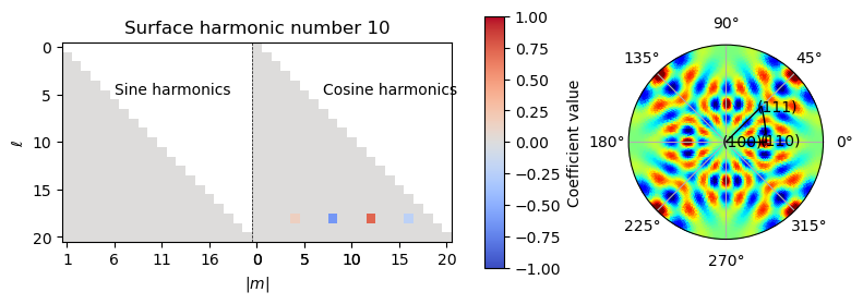
The modes are linear combinations of spherical harmonics coefficients at a fixed \(\ell\) that give symmetric functions:

For cubic, these modes are always linear combinations of cosine-terms with \(m\) divisible by 4. For other point groups the modes are single coefficients.

# PLot an example surface harmonic
mode_number = 10

# Convert the coefficients into a format nice for plotting
coeff_array_unwrapped = np.zeros((ell_max+1, ell_max*2+1))
coeff_array_unwrapped[...] = np.nan
example_mode = cube_harmonics[mode_number]
for ell in range(ell_max+1):
    coeff_array_unwrapped[ell, ell_max:(ell_max+ell+1)] = 0
    coeff_array_unwrapped[ell, 0:ell] = 0
ell = example_mode.ell
coeff_array_unwrapped[ell, ell_max:(ell_max+ell+1)] = example_mode.coefficients[ell:]
coeff_array_unwrapped[ell, 0:ell] = example_mode.coefficients[:ell]

# PLot coefficient matrix with nice formatting
fig = plt.figure(figsize = (9, 3))
gs = gridspec.GridSpec(1, 4, figure=fig, width_ratios=[2.0, 0.1, 0.3, 1])
############# DENSITY SLICE #####################################
ax = fig.add_subplot(gs[0,0])
img = plt.imshow(coeff_array_unwrapped, vmin = -1, vmax = 1, cmap = 'coolwarm')
plt.ylabel(r'$\ell$'); plt.xlabel('$|m|$')
plt.xticks(np.append(np.arange(0, 32, 5), np.arange(ell_max, ell_max + 32, 5)), np.append(np.arange(1, 32, 5), np.arange(0, 33, 5)))
plt.plot([ell_max-0.5]*2, [-0.5, ell_max+0.5], 'k--', linewidth = 0.5)
plt.text(5, 5, 'Sine harmonics')
plt.text(7+ell_max, 5, 'Cosine harmonics')
plt.title(f'Surface harmonic number {mode_number}')
cbar = fig.colorbar(img, cax = fig.add_subplot(gs[0,1]), label = 'Coefficient value')

# PLot example inverse pole figure
ax = fig.add_subplot(gs[0,3], polar = True)
map_theta = np.linspace(0, np.pi/2, 91)
map_phi = np.linspace(0, np.pi*2, 361)
map_intens = map_single_l(ell, example_mode.coefficients, map_theta, map_phi)
img = ax.pcolormesh(map_phi, np.tan(map_theta/2), map_intens, edgecolors = 'face', rasterized = True, cmap = 'jet', vmin = -2.5, vmax = 2.5)
plt.yticks([])
plot_tools.polefigure.plot_cubic_asym_outline(ax)
plt.savefig('../img/cubic_surface_harmonic.png')

plt.show()

Initialize an object representing the ODF model from the list of surface harmonics.

odf = odfs.Harmonics(ell_max, cube_harmonics, point_group=point_groups.cubic)
print(f'Model uses {odf.n_modes} modes')

Model uses 362 modes

Define lattice matrix used to convert Miller indicies into \(\mathbf{h}\)-vectors and initialize the forward model of the reconstruction problem. In the cubic system, this is not strictly necessary, but we do it anyways to build good habits.

A, B = cubic()
h_vectors = [B @ hkl for hkl in hkl_list]

Now we define the full forward model, which is composition of a pole-figure transform and a Radon transform:

The pole figure transform is performed by a list of pre-computed arrays containging the scattering intensities of the individual texture basis function modes.

The Radon transform is performed by the mumott implementation.

basis_function_matrices = []
for rotation_index in range(data_slice.shape[0]):
    basis_function_matrices.append(odf.evaluate_pfmatrix(coordinates[rotation_index, 0, 0], h_vectors))

model = FromArrayModel(basis_function_matrices, geom_slice)

4. Run actual reconstruction

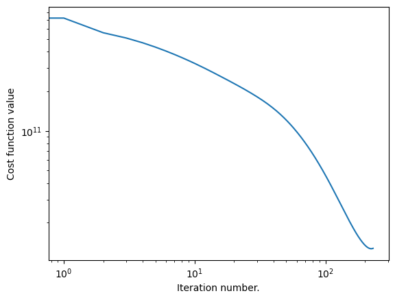
Define an optimizer object and run the optimization. As we are working on Harmonics, we must remember to set the nonneg parameter to False and L1-regularization cannot be used.

The algorithm used here is typically unstable with the harmonics (the problem seems to be rank deficient) but if we stop optimization early, we still get resonable results in many cases.

optimizer = FISTA(model, data_slice, weights=weigth_slice, nonneg=False, maxiter=230) # (I picked the number of iterations
                                                                                      #  to just see the start of instability)
x, convergence_curve = optimizer.optimize()

fig = plt.figure()
plt.loglog(convergence_curve)
plt.xlabel('Iteration number.')
plt.ylabel('Cost function value')
plt.show()

Estimating largest safe step size

Matrix norm estimate = 4.08E+05:  30%|███       | 3/10 [00:00<00:02,  3.31it/s]
Loss = 1.27E+10: 100%|██████████| 230/230 [00:53<00:00,  4.30it/s]

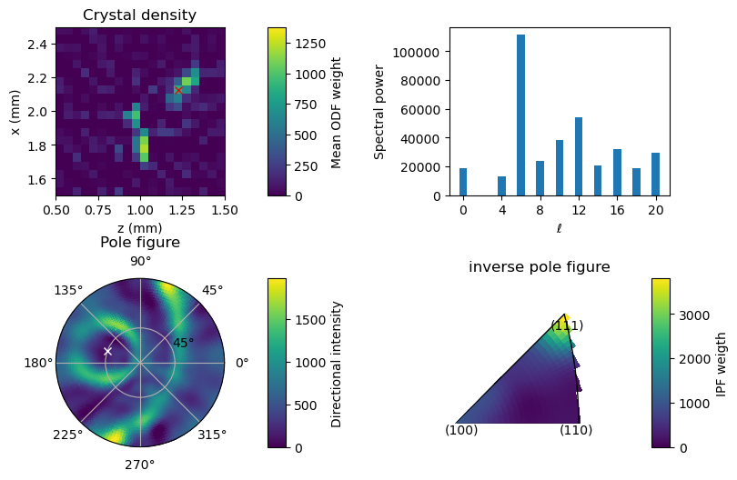
5. Basic plots of the reconstruction

We have different notebooks demonstrating ways to visualize the reconstructions. Here we just plot the density and some (inverse)-pole figures.

fig = plt.figure(figsize = (9,6))

coeffs = x;
example_voxel = (18, 0, 24)
ipf_direction = (45*np.pi/180, 160*np.pi/180) # This is the direction in which the inverse pole-figure will be computed
ipf_xyz = [np.cos(ipf_direction[1])*np.sin(ipf_direction[0]),
           np.sin(ipf_direction[1])*np.sin(ipf_direction[0]),
           np.cos(ipf_direction[0]),]
pcolor_opts = {'edgecolors':'face', 'vmin':0}
imshow_opts = {'extent':(0,3,0,3), 'vmin':0.0}#{'vmax':0.0005, 'extent':(0,3,0,3)}

gs = gridspec.GridSpec(3, 5, figure=fig, width_ratios=[0.7, 0.06, 0.4, 0.6, 0.06], height_ratios=[1, 0.2, 1,])
############# DENSITY SLICE #####################################
ax = fig.add_subplot(gs[0,0])
img = plt.imshow(coeffs[:,example_voxel[1],:,0], **imshow_opts)
ax.set_xlim(0.5,1.5); ax.set_ylim(1.5,2.5)
plt.plot(example_voxel[2]*0.05+0.025, 3-example_voxel[0]*0.05+0.025, 'rx')
ax.set_xlabel('z (mm)'); ax.set_ylabel('x (mm)')
plt.title('Crystal density')
cax = fig.add_subplot(gs[0,1])
fig.colorbar(img, cax = cax, label = 'Mean ODF weight')

# ##############  SINGLE PIXEL POLEFIGURE ########################
ax = fig.add_subplot(gs[2,0], polar=True)
voxel_coeffs_symmetrized = coeffs[example_voxel[0], example_voxel[1], example_voxel[2],:]
polefigure, theta_grid, phi_grid = odf.make_polefigure_map(voxel_coeffs_symmetrized, [1, 1, 0])
img = ax.pcolormesh(phi_grid, np.tan(theta_grid/2), polefigure, **pcolor_opts)
ax.set_yticks([np.tan(ii*np.pi/8) for ii in range(1,2)])
ax.set_yticklabels(['45°'])
ax.yaxis.label.set_color('w')
plt.title('Pole figure')
plt.plot(ipf_direction[1], np.tan(ipf_direction[0]/2), 'wx')
cax = fig.add_subplot(gs[2,1])
fig.colorbar(img, cax = cax, label = 'Directional intensity')

# ##############  SINGLE PIXEL INVERSE POLEFIGURE ########################
ax = fig.add_subplot(gs[2,3], polar=True)
inverse_polefigure, theta_grid, phi_grid = odf.make_inverse_polefigure_map(voxel_coeffs_symmetrized, ipf_xyz)

# Crop inverse pole figure to asymmetric zone
inverse_polefigure[phi_grid>45*np.pi/180] = np.nan # Line from [001] to [111]
inverse_polefigure[phi_grid<0] = np.nan # Line from [001] to [101]
grid_x = np.cos(phi_grid)*np.sin(theta_grid)
grid_z = np.cos(theta_grid)
inverse_polefigure[grid_x > grid_z] = np.nan

img = ax.pcolormesh(phi_grid, np.tan(theta_grid/2), inverse_polefigure, **pcolor_opts)
ax.set_yticks([np.tan(ii*np.pi/8) for ii in range(1,2)])
ax.set_yticklabels(['45°'])
ax.yaxis.label.set_color('w')
plt.title('inverse pole figure')
plt.xlim(0, 46*np.pi/180); plt.ylim(0, np.tan(59*np.pi/180/2))
plt.axis('off')
plot_tools.polefigure.plot_cubic_asym_outline(ax)
cax = fig.add_subplot(gs[2,4])
fig.colorbar(img, cax = cax, label = 'IPF weigth')

# #################### POWER SPECTRAL DENSITY  ######################
ax = fig.add_subplot(gs[0,3:])
power_spectrum = np.zeros(ell_max//2 + 1)
mask = coeffs[...,0] > 1
for modenumber in range(odf.n_modes):
    ell = odf.mode_coefficients[modenumber].ell
    power_spectrum[ell//2] += np.mean(coeffs[mask,modenumber]**2)

plt.bar(np.arange(0, ell+1, 2), power_spectrum)
plt.xticks(np.arange(0, ell_max+1, 4))
plt.xlabel(r'$\ell$'); plt.ylabel('Spectral power')
plt.show()

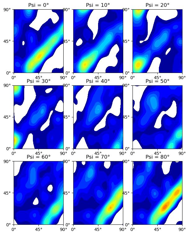
For closer comparison with the RBF reconstructions, we calculate Euler angle sections of a single voxel.

# Euler-sections of single-pixel texture
GSH_coeffs = odf.make_GSH_coeffs(voxel_coeffs_symmetrized)
Psi = np.linspace(0, np.pi/2, 9, endpoint=False)
Theta = np.linspace(0, np.pi/2, 51, endpoint=False)
Phi = np.linspace(0, np.pi/2, 51, endpoint=False)

ODF_map, (Psi_map, Theta_map, Phi_map) = GSH_mapper(GSH_coeffs, odf.ell_max,
                                                    euler_angles_tuple = (Psi, Theta, Phi))
ODF_map = ODF_map / GSH_coeffs[0][0,0]

plt.figure(figsize = (7, 9))
for ii in range(9):
    plt.subplot(3,3,ii+1)
    plt.contourf(ODF_map[ii,:,:], extent = (0, 90, 0, 90),
                 levels=np.linspace(0, 10, 21), cmap='jet')
    plt.title(f'Psi = {Psi_map[0, 0, ii]*180/np.pi:.0f}°')
    ticks = [0, 45, 90]; labels = ['0°', '45°', '90°']
    plt.xticks(ticks, labels=labels)
    plt.yticks(ticks, labels=labels)
    plt.savefig('../img/euler_sections_GSH.png')
plt.show()

/tmp/ipykernel_3116744/3932168186.py:7: UserWarning: Gimbal lock detected. Setting third angle to zero since it is not possible to uniquely determine all angles.
  ODF_map, (Psi_map, Theta_map, Phi_map) = GSH_mapper(GSH_coeffs, odf.ell_max,
100%|██████████| 21/21 [00:04<00:00,  4.48it/s]