Grain-by-grain workflow
While texture-tomography was first suggested as a way to reconstruct XRD-CT data from very small grained materials, where each reconstruction voxel contains a large number of grains, it has turned out that it performs well on deformed large grained materials as well.
The standard RBF workflow can sometimes give acceptable grain maps for difficult samples where even state-of-the-art scanning-3D-XRD algorithms are not thought to perform well. However, the orientation resolution is limited by the grid nearest neighbor spacing which is hard to get much lower than about \(5^\circ\) before running into computational problems due to the size of the ODF expansion.
Inspired by 6D-DCT, I have implemented a separate workflow which reconstructs grains one at a time, where the voxel-by-voxel ODF is modeled by a finely spaced grid of orientations centered on the average orientation of the grain.
This workflow enables reconstructions with better orientation resolution than the normal texture-tomography workflow and maintains better ability to handle deformed materials than s3DXRD. This comes at the cost of a slow reconstruction with a lot of tunable parameters.
This jupyter notebook documents the complicated workflow in the following steps:
Simulating a dataset
Normal RBF reconstruction
Grain segmentation
Single grain basis funcitons
Grain-by-grain reconstruction
[1]:
import matplotlib.pyplot as plt
import matplotlib as mpl

import numpy as np
from scipy.spatial.transform import Rotation as R
from scipy.ndimage import find_objects
from tqdm import tqdm

from odftomo.io.make_2d_geometry import make_2D_mumott_geometry
from odftomo.io.mumott_fileformat_loader import get_probed_coordinates
from odftomo.texture import grids, point_groups, odfs
from odftomo.tomography_models import FromArrayModel, OnTheFlyModel
from odftomo.crystallography import cubic
from odftomo.optimization import FISTA
from odftomo.analysis.segmentation import find_texture_components, grain_segmentation
from odftomo import plot_tools
from mumott.methods.projectors import SAXSProjector as Projector
INFO:Setting the number of threads to 4. If your physical cores are fewer than this number, you may want to use numba.set_num_threads(n), and os.environ["OPENBLAS_NUM_THREADS"] = f"{n}" to set the number of threads to the number of physical cores n.
INFO:Setting numba log level to WARNING.
1. Simulating a dataset
The grain-by-grain reconstruction only does well with quite fine sampling in the tomographic rotation. (I have been working with \(0.5^\circ\) experimentally and \(1^\circ\) in this simulation.)
This unfortunately means that the datasets I have published so far cannot be used so this demonstration uses simulated data. You unfortunately just have to trust me for now that it also works well with real data. I will try to upload something better soon!
The data is simulated with a model consisting of spatially varying orientation field with a symmetric Gaussian texture in each voxel with a \(\sigma = 0.02\mathrm{rad}\) orientation spread.
[2]:
# Create a 2D geometry object
rotation_angles = np.linspace(0, 180, 180, endpoint = False)
azimuthal_angles = np.linspace(0, 360, 360, endpoint = False)
geometry = make_2D_mumott_geometry(50, rotation_angles, azimuthal_angles)

A, B = cubic()
hkl_list = [(1, 1, 1), (2, 0, 0), (2, 2, 0), (3, 1, 1)]
two_theta_list = [2 * np.arcsin(np.sqrt(hkl[0]**2+hkl[1]**2+hkl[2]**2)/20) * 180 / np.pi for  hkl in hkl_list]
h_vectors = [(B @ hkl)/np.linalg.norm(B @ hkl)  for hkl in hkl_list]

coordinates = []
for hkl_index in range(len(hkl_list)):
    geometry.two_theta  = two_theta_list[hkl_index] * np.pi / 180
    coordinates.append(get_probed_coordinates(geometry)[:, :, 0, :])

coordinates = np.stack(coordinates, axis=-1)
coordinates = coordinates.transpose((0, 1, 3, 2))[:, np.newaxis, np.newaxis, :, :]
[3]:
# Make a sample consisting of 4 grains in a simple geometric configuration
x = np.arange(geometry.volume_shape[0])
z = np.arange(geometry.volume_shape[2])
x, z = np.meshgrid(x, z, indexing='ij')

disc = ((x-24.5)**2 + (z-24.5)**2) < 24**2
phi = np.arctan2(z-24.5, x-24.5)
grain_label = np.floor((phi+np.pi/4) % (2*np.pi) / (np.pi/2)).astype(int)
grain_label[~disc] = -1
[4]:
# Make an orientation_field
grain_mean_orientations = R.from_rotvec([[ 0.3, 0.1, 0.2],
[-0.5, -0.45,-0.50],
[-0.6, 0.5, 0.3],
[ 0.3, -0.05, -0.2],])
shape_2d = (geometry.volume_shape[0], geometry.volume_shape[2])
low_frequency_noise = np.zeros((*shape_2d, 3), dtype=complex)
noise_bl = 2
low_frequency_noise[:noise_bl, :noise_bl, :] = np.random.rand(noise_bl,noise_bl,3) + 1j * np.random.rand(noise_bl,noise_bl,3) - 0.5 - 0.5j
low_frequency_noise[:noise_bl, -noise_bl:, :] = np.random.rand(noise_bl,noise_bl,3) + 1j * np.random.rand(noise_bl,noise_bl,3) - 0.5 - 0.5j
low_frequency_noise[-noise_bl:, -noise_bl:, :] = np.random.rand(noise_bl,noise_bl,3) + 1j * np.random.rand(noise_bl,noise_bl,3) - 0.5 - 0.5j
low_frequency_noise[-noise_bl:, :noise_bl, :] = np.random.rand(noise_bl,noise_bl,3)+ 1j * np.random.rand(noise_bl,noise_bl,3) - 0.5 - 0.5j
low_frequency_noise = np.real(np.fft.fftn(low_frequency_noise, axes = (0,1)))
gt_orientation_field = np.zeros((*shape_2d, 3))
for grain_index in range(4):
grain_mask = grain_label==grain_index
ori = grain_mean_orientations[grain_index] * R.from_rotvec(low_frequency_noise[grain_mask]*5e-2)
gt_orientation_field[grain_mask, :] = ori.as_rotvec()
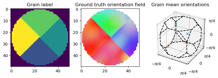
# PLot simulation ground truth
ipf_direction = np.array([0,1,0,])
ipf_color_gt = plot_tools.IPF_color(gt_orientation_field, ipf_direction, 'cubic')
ipf_color_gt[~disc,:]=1
fig = plt.figure(figsize = (9,3))
plt.subplot(1,3,1)
plt.imshow(grain_label)
plt.title('Grain label')
plt.subplot(1,3,2)
plt.imshow(ipf_color_gt)
plt.title('Ground truth orientation field')
ax = plt.subplot(1,3,3,projection='3d')
for grain_ori in grain_mean_orientations:
plt.plot(*grain_ori.as_rotvec(), 'x')
plt.title('Grain mean orientations')
plot_tools.plot_asym_zone_outline(ax, 'cubic')
plt.show()
[5]:
# Make simulated data
projector = Projector(geometry) # Stand-alone radon transform
simulation_sigma = 0.02

sim_data_array = np.zeros((len(geometry), *geometry.projection_shape, len(azimuthal_angles), len(hkl_list)))
gt_orientations = R.from_rotvec(gt_orientation_field.reshape((-1,3)))
for rotation_index in tqdm(range(len(geometry))):
    for symmetry_element in point_groups.cubic:
        for hkl_index in range(len(hkl_list)):
            exact_direction = (gt_orientations * symmetry_element).apply(h_vectors[hkl_index]).reshape((*shape_2d, 3))
            cos_distance = np.abs(np.einsum('pi,xzi->xzp', coordinates[rotation_index, 0, 0, :, hkl_index,:], exact_direction))
            voxel_scattering = np.exp(4*(cos_distance-1)/2/simulation_sigma**2)
            voxel_scattering[~disc, :] = 0
            sim_data_array[rotation_index, :, 0, :, hkl_index] += projector.forward(voxel_scattering[:,np.newaxis,:,:], [rotation_index])[0,:,0,:]
100%|██████████| 180/180 [17:23<00:00, 5.80s/it]
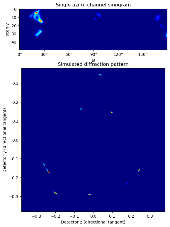
[6]:
# PLot simulated data
hkl_index = 2
azim_index = 35

fig = plt.figure(figsize = (9,9))
gs = mpl.gridspec.GridSpec(2, 1, figure=fig, height_ratios=(1, 3.5))

ax = fig.add_subplot(gs[0, 0])
plt.imshow(sim_data_array[:,:,0,azim_index,hkl_index].T, cmap='jet')
plt.ylabel('scan y')
plt.xlabel(r'$\omega$')
ax.set_xticks(np.arange(0, 180, 30))
ax.set_xticklabels([f'{v:.0f}°' for v in rotation_angles[np.arange(0, 180, 30)]])
plt.title('Single azim. channel sinogram')

ax = fig.add_subplot(gs[1, 0])
scatt_data = sim_data_array[0, 15, 0, :, :]
cmap = mpl.cm.get_cmap('jet')
plot_tools.plot_simulated_diffraction_pattern(geometry, np.array(two_theta_list)*np.pi/180,
                                              scatt_data=scatt_data, ax = ax, cmap=cmap, bg_color=cmap(0)[:3])
ax.set_xlim(-0.38, 0.38)
ax.set_ylim(-0.38, 0.38)
plt.ylabel('Detector y (directional tangent)')
plt.xlabel('Detector z (directional tangent)')
plt.title('Simulated diffraction pattern')
plt.show()
/tmp/ipykernel_1479728/353676136.py:18: MatplotlibDeprecationWarning: The get_cmap function was deprecated in Matplotlib 3.7 and will be removed in 3.11. Use ``matplotlib.colormaps[name]`` or ``matplotlib.colormaps.get_cmap()`` or ``pyplot.get_cmap()`` instead.
  cmap = mpl.cm.get_cmap('jet')
2. Normal RBF reconstruction
The grain-by-grain reconstruction needs as input a bounding box and a mean orientation of each grain. This amounts to a solution of the indexing problem, which is to assign a grain ID to each diffraction peak in the dataset.
This is probably possible by with existing 3D-XRD algorithms, but here we run a normal RBF texture tomography reconstruction to get the orientation field and do grain segmentation.
The RBF workflow is documented elsewhere, so here we just run through it quickly.
[7]:
# Define a model of the ODF
grid_resolution_parameter = 31
recon_sigma = 0.05
grid = grids.hopf_grid(grid_resolution_parameter, point_groups.cubic)
odf = odfs.GaussianRBF(grid, point_groups.cubic, recon_sigma)
basis_function_arrays = odf.compute_polefigure_matrices_parallel(coordinates, h_vectors, num_processes=4)
RBF_model = FromArrayModel(basis_function_arrays, geometry)
Starting parallel computation of polefiugres.
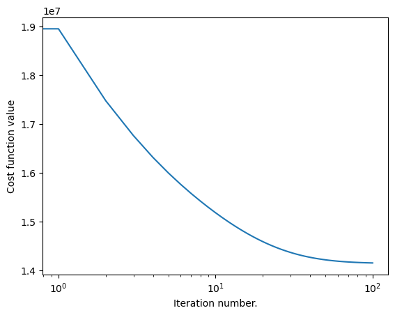
[8]:
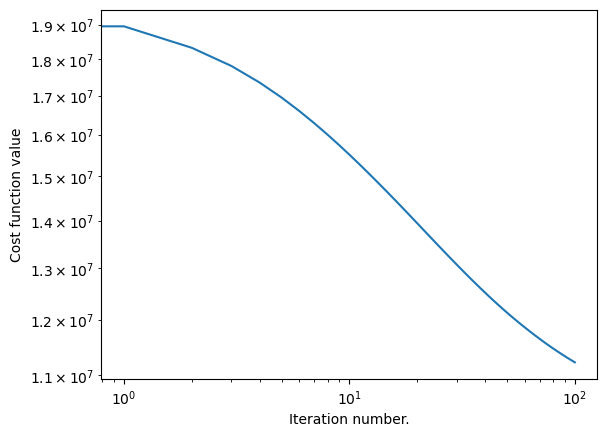
# Run RBF reconstruction
solidangle_factor = np.abs(np.cos(np.deg2rad(azimuthal_angles)))[np.newaxis, np.newaxis, np.newaxis, :, np.newaxis] * np.ones(sim_data_array.shape)
optimizer = FISTA(RBF_model, sim_data_array, weights=solidangle_factor, maxiter=100, volume_mask=disc[:, np.newaxis, :])
RBF_coefficients, convergence_curve = optimizer.optimize()

plt.figure()
plt.loglog(convergence_curve)
plt.xlabel('Iteration number.')
plt.ylabel('Cost function value')
plt.show()
Estimating largest safe step size
Matrix norm estimate = 6.42E+10:  30%|███       | 3/10 [00:26<01:02,  8.96s/it]
Loss = 1.12E+07: 100%|██████████| 100/100 [11:30<00:00,  6.91s/it]
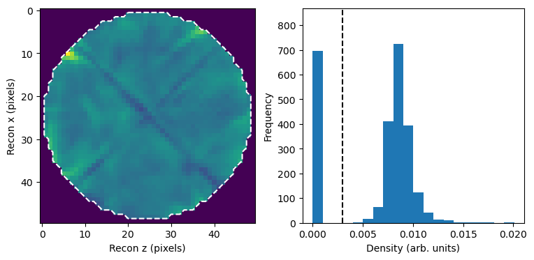
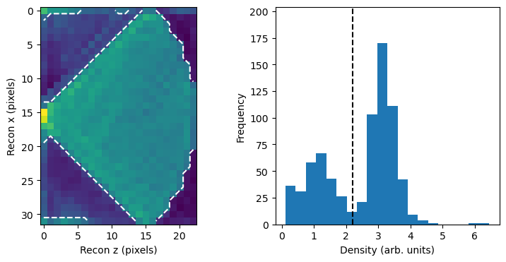
[9]:
# Pick a threshold value to determine what pixels to plot.
mask_threshold = 0.003

plt.figure(figsize = (9, 4))
dens = np.sum(RBF_coefficients, axis = -1)
mask = dens > mask_threshold

plt.subplot(1,2,1)
plt.imshow(dens[:,0,:])
plt.contour(mask[:,0,:], levels = [0.5], colors=[(1,1,1)],linestyles='dashed')
plt.xlabel('Recon z (pixels)'); plt.ylabel('Recon x (pixels)');

plt.subplot(1,2,2)
freq = plt.hist(dens.flatten(), bins = 20)[0]
plt.ylim(0, np.max(freq)*1.2)
plt.plot([mask_threshold]*2, [0, np.max(freq[5:])*1.2], 'k--')
plt.xlabel('Density (arb. units)')
plt.ylabel('Frequency')
plt.show()
[21]:
# Compute some quantities for plotting
pole_figure_hkl = np.array([0, 0, 1])
coeffs_2d = RBF_coefficients[:,0,:,:]
example_voxel = (10, 0, 30)
stepsize = 1
pcolor_opts = {'edgecolors':'face', 'vmin':0, 'rasterized':True}
imshow_opts = {'extent':(0,coeffs_2d.shape[1]*stepsize,coeffs_2d.shape[0]*stepsize,0)}

def tomogram_set_axes(ax):
    ax.set_xlabel('z (pixels)')
    ax.set_ylabel('x (pixels)')
    ax.grid()

# Compute the plotted quantities
mask_2d = np.sum(coeffs_2d, axis = -1) > mask_threshold

# Compute max direction IVP colormap
main_orientation_tomogram = odf.main_orientation(RBF_coefficients)
ivp_map_rgb = plot_tools.IPF_color(main_orientation_tomogram, ipf_direction, 'cubic')[:, 0, :]
ivp_map_rgb[~mask_2d, :] = 1

# Compute approximate texture index
J = np.sqrt(np.var(coeffs_2d, axis = -1)) / np.mean(coeffs_2d, axis = -1)
J[~mask_2d] = np.nan
# Compute a pole-figure of a single voxel
voxel_coeffs = RBF_coefficients[example_voxel[0], example_voxel[1], example_voxel[2],:]
polefigure, theta_grid, phi_grid = odf.make_polefigure_map(voxel_coeffs, B @ pole_figure_hkl)
/tmp/ipykernel_1479728/81798759.py:24: RuntimeWarning: invalid value encountered in divide
  J = np.sqrt(np.var(coeffs_2d, axis = -1)) / np.mean(coeffs_2d, axis = -1)
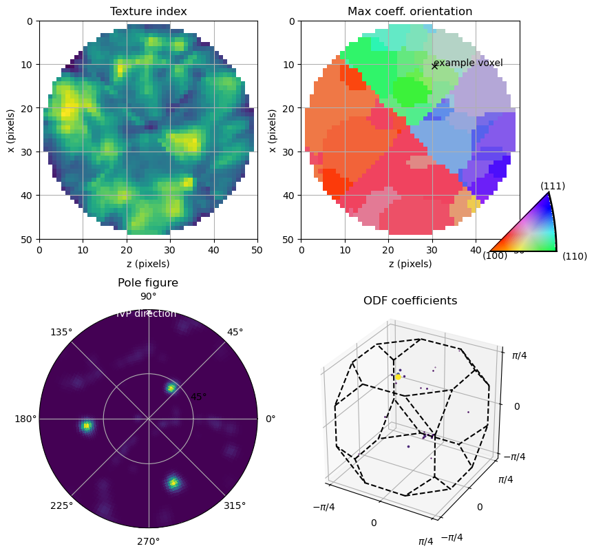
[22]:
# Build the plot
fig = plt.figure(figsize = (9, 10))

# PLot IVP-map
ax = plt.subplot(2,2,2)
ax.imshow(ivp_map_rgb, **imshow_opts)
ax.plot((example_voxel[2]+0.5)*stepsize, (example_voxel[0]+0.5)*stepsize, 'kx')
ax.text((example_voxel[2]+0.5)*stepsize - 0.2, (example_voxel[0]+0.5)*stepsize - 0.1, 'example voxel', color = 'k')
tomogram_set_axes(ax)
ax.set_title('Max coeff. orientation')
ax = fig.add_subplot([0.85, 0.5, 0.15, 0.15], polar = True)
plot_tools.make_color_legend(ax, 'cubic')

# Plot texture index
ax = plt.subplot(2,2,1)
img = ax.imshow(J, **imshow_opts)
tomogram_set_axes(ax)
ax.set_title('Texture index')

# PLot pole figure
ax = plt.subplot(2,2,3, polar=True)
img = ax.pcolormesh(phi_grid, np.tan(theta_grid/2), polefigure, **pcolor_opts)
ax.set_yticks([np.tan(ii*np.pi/8) for ii in range(1,2)])
ax.set_yticklabels(['45°'])
ax.yaxis.label.set_color('w')
ax.set_title('Pole figure')
if ipf_direction[2] < 0.0:
    ipf_direction = -ipf_direction
IVP_map_theta = np.arctan2(np.sqrt(ipf_direction[0]**2+ipf_direction[1]**2), ipf_direction[2])
IVP_map_phi = np.arctan2(ipf_direction[1], ipf_direction[0])
ax.plot(IVP_map_phi, np.tan(IVP_map_theta/2), 'wx')
ax.text(IVP_map_phi+0.3, np.tan(IVP_map_theta/2), 'IVP direction',color = 'w')

# PLot ODF modes in Rodriguez-vector representation
ax = plt.subplot(2,2,4, projection='3d')
plot_tools.plot_orientation_coeffs(voxel_coeffs, odf.grid, ax, point_group_string='cubic')
ax.set_title('ODF coefficients')
fig.show()
3 - Grain segmentation
To get the grain positions and orientation, we run through the usual grain-segmentation workflow for RBF reconstructions.
First we perform pixel-by-pixel ODF clustering:
[ ]:
# Find texture components in each voxel
texture_component_tomogram = find_texture_components(
    RBF_coefficients,
    odf,
    density_threshold = mask_threshold,
    texture_component_radius = 20.0,
)

print(f'In total {np.sum(texture_component_tomogram!=0)} texture components were found')
print(f'with a maximum of {np.max(np.sum(texture_component_tomogram!=0, axis = -1))} texture components in a single voxel.')
/das/home/carlse_m/grids_in_so3/odftt/analysis/grid_tools.py:112: RuntimeWarning: invalid value encountered in arccos
  dist_this = np.arccos(2*np.abs(np.einsum('ik,k->i',
 44%|████▎     | 1088/2500 [00:30<00:41, 33.93it/s]
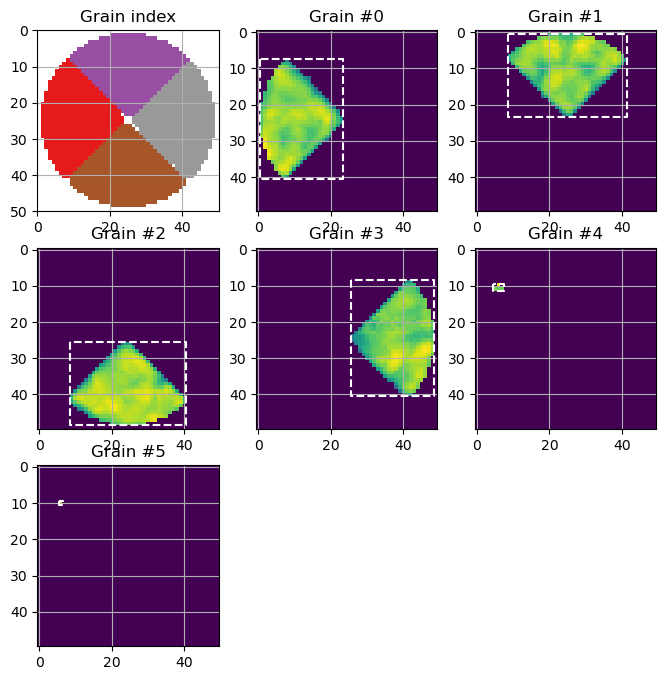
Then texture components in neighboring pixels and with similar orientations are grouped into grains.
[25]:
sorted_grains_list = grain_segmentation(
    texture_component_tomogram,
    distance_threshold=5.0,
    point_group=odf.point_group,
)

print(f'The texture components were segmented into {len(sorted_grains_list)} grains.')
The texture components were segmented into 6 grains.
[26]:
# Make a map of grain-indexes of grain with highest density
grain_number = 0
grain_index = np.zeros(geometry.volume_shape)
main_grain_dens = np.zeros(geometry.volume_shape)
for index, grain in enumerate(sorted_grains_list[:30]):
    where = grain.density > main_grain_dens
    grain_index[where] = index
    main_grain_dens[where] = grain.density[where]
grain_index[main_grain_dens==0] = np.nan

fig = plt.figure(figsize = (8, 8))
ax = plt.subplot(3,3,1)
plt.imshow(grain_index[:,0,:]%10,**imshow_opts, cmap = 'Set1', interpolation = 'nearest')
plt.title('Grain index')
ax.grid()

for grain in sorted_grains_list[:8]:
    ax = plt.subplot(3,3,grain_number+2)
    ax.imshow(np.sum(grain.density, axis=1))
    ax.set_title(f'Grain #{grain_number}')
    ax.grid()
    bbox = grain.bbox_voxel
    ax.plot(np.array([bbox[4], bbox[4], bbox[5], bbox[5], bbox[4]])-0.5,
            np.array([bbox[0], bbox[1], bbox[1], bbox[0], bbox[0]])-0.5, '--w')
    grain_number+=1
plt.show()
4. Single grain basis functions
Before we move on to the reconstuctions, we introduce the basis-functions in a bit more detail.
When we want to model a small part of orientation space, we can sometimes simplify things by linearizing rotations. A sketch of a derivation starts with the aproximation of rotation matrixes of small rotation by skew-symmetric matrixes of the shape:
where \(\mathbf{r} = [r_x, r_y, r_z]^{\mathrm{T}}\) is a 3-vector (equal to the Rodriguez vector to first order) that parametrizes the rotations. In this aproximation, rotation of a vector \(\mathbf{v}\) is replaced by a cross product:
where \(\times\) is the vector cross product. And composition of rotation matrixes aproximatelty becomes vector-addition:
The idea we will make use of is that the integral used to compute the pole-figure transform can be approximated by a straight line in \(\mathbf{r}\)-space.
where we are using Bunge’s notation with lattice-space unit vectors \(\mathbf{h}\), sample-space vectors \(\mathbf{y}\) and \(\langle \mathbf{h}, \mathbf{y} \rangle = \{g\in\mathrm{SO}(3):\,\mathbf{y}=g\mathbf{h} \}\).
The range for \(s\) is not important if we are considering functions in \(\mathrm{SO}(3)\) that are only non-zero for small rotations.
Because the foward model is now a line-integral, we can use efficient algorithms from CT instead of pre-computed matrixes.
The last detail is to generalize our approximation for small rotations (a small region around \(g=e\)) to an approximation for a small region around an arbitrary orientation \(g= g_0\). This is done by a right-sided shift of the definitions above:
which means all \(\mathbf{h}\) vectors in the above equations should be replaced by \(g_0\mathbf{h}\).
Let’s set up such a model for one of the grains in the simulated sample. Aside from the real-space bounding box and the mean orientation which we get from the RBF reconstruction, there are two additional parameters: an orientation space range in radians and a number of steps along the box edge.
[27]:
# Choose which plot to reconstruct
grain_index = 3
# For the comparison plots below, you also need to tell which ground-truth grain
# label this coresponds to.
gt_grain_label = 1

# Make the single-grain ODF model
grain = sorted_grains_list[grain_index]
grid_range = 0.15 # Half range of box in radians (approx. largest misorientation in grain)
grid_scale = 15 # Number of steps in each direction
grain_odf = odfs.SingleGrain(grain.COM_ori, grid_range, grid_scale, point_groups.cubic)
[28]:
# Make a geometry object corresponding to single grain ROI
# Grain center position relative to full tomogram center
bbox = grain.bbox_voxel
offset_xyz = np.array([0.5*(bbox[0]+bbox[1])-geometry.volume_shape[0]/2,
                       0.5*(bbox[2]+bbox[3])-geometry.volume_shape[1]/2,
                       0.5*(bbox[4]+bbox[5])-geometry.volume_shape[2]/2,])

# Offset projected onto the raster-scan direction
offset_j = []
for rotation in geometry.rotations:
    offset_j.append(-np.dot((rotation @ offset_xyz), geometry.j_direction_0))
offset_j = np.array(offset_j)

from copy import deepcopy
grain_geometry = deepcopy(geometry)
grain_geometry.j_offsets += offset_j
grain_geometry.volume_shape = [bbox[1]-bbox[0], 1, bbox[5]-bbox[4]]
[30]:
# Utility for rodriguez vector plotting
def plot_orientation_bbox(ax):
    box_edges = np.array([[-1, -1, -1], [-1, -1, 1], [-1, 1, 1], [-1, 1, -1], [-1, -1, -1],
                          [1, -1, -1], [1, -1, 1], [-1, -1, 1], [1, -1, 1], [1, 1, 1],
                          [-1, 1, 1], [1, 1, 1], [1, 1, -1], [-1, 1, -1], [1, 1, -1], [1, -1, -1],])

    box_half_edge = grid_range
    box_edges = (R.from_rotvec(box_half_edge * box_edges) * grain.COM_ori).as_rotvec()
    ax.plot(box_edges[:,0], box_edges[:,1], box_edges[:,2], 'k')
    ax.set_aspect('equal')

grain_mask = grain.density > 0.0
rots = R.from_rotvec(grain.rotvec_array[grain_mask])

# Make colours
grain_rotvec_map = np.ones(grain.rotvec_array.shape)
grain_rotvec_map[grain_mask] = rots.as_rotvec()
grain_IPF_rgb = plot_tools.IPF_color(grain_rotvec_map[:, 0, :], ipf_direction, 'cubic')
grain_IPF_rgb[~grain_mask[:, 0, :]] = 1

fig = plt.figure(figsize = (9,9))
# Full symeetric zone with ODF and bbox
ax = plt.subplot(2, 2, 1, projection = '3d')
ax.scatter(grain.rotvec_array[grain_mask,0], grain.rotvec_array[grain_mask,1], grain.rotvec_array[grain_mask,2],
           c = grain_IPF_rgb[grain_mask[:,0,:], :], s = 5)
plot_tools.plot_asym_zone_outline(ax, 'cubic')
ax.set_title('Grain ODF with bbox')
plot_orientation_bbox(ax)

# RBF grid
ax = plt.subplot(2, 2, 3, projection = '3d')
RBF_grid_rotvecs = (odf.grid * grain_odf.average_orientation.inv()).as_rotvec()
in_bbox = np.all(np.abs(RBF_grid_rotvecs) <= grid_range * 1.0, axis=1)
RBF_grid_rotvecs = odf.grid.as_rotvec()
ax.scatter(RBF_grid_rotvecs[in_bbox,0], RBF_grid_rotvecs[in_bbox,1], RBF_grid_rotvecs[in_bbox,2],
           c = 'k', s = 10, alpha = 1)
plot_orientation_bbox(ax)
ax.set_title('RBF grid-points inside bbox')

# IPF map
ax = plt.subplot(2, 2, 2)
plt.imshow(grain_IPF_rgb)
ax.set_title('Single grain IPF-map')
ax.plot(np.array([bbox[4], bbox[4], bbox[5], bbox[5], bbox[4]])-0.5,
        np.array([bbox[0], bbox[1], bbox[1], bbox[0], bbox[0]])-0.5, '--k')

# Single-grain grid
ax = plt.subplot(2, 2, 4, projection = '3d')
grid_rotvecs = grain_odf.rotation_grid().as_rotvec()
ax.scatter(grid_rotvecs[:,0], grid_rotvecs[:,1], grid_rotvecs[:,2], s = 0.3, c='k')
ax.set_title('Single grain grid')
plot_orientation_bbox(ax)

plt.savefig('../img/single_grain_grid.png')
plt.show()
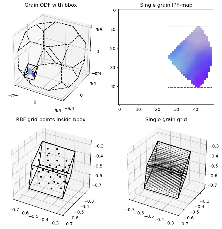
Figure caption: a) shows the pixel mean orientations of the grain of interest. b) shows the mean orientation in IPF map and the bounding box, c) and d) shows a zoomed in region of rotation space with the bounding box and the RBF and single-grain orientation grids respectively.
5. Grain-by-grain reconstruction
With a model set up, we can now try to reconstruct a single grain. We don’t try to filter out the peaks from other grains, we just fit to the full dataset and hope the local-tomography figures the rest out.
For less perfect data, we often find that the reconstructions need L-1 regularization, otherwise they develop large artefacts at the edges of both the real- and reciprocal space bounding boxes. This means we need to perform a sweep over the regularization parameter which costs a lot of computer time. It seem that once a good parameter is found for one grain, it can be re-used for the rest of the grains in the same sample.
[31]:
grain_model = OnTheFlyModel(grain_odf, grain_geometry, coordinates, h_vectors)
optimizer_2 = FISTA(grain_model, sim_data_array, maxiter=100, weights=solidangle_factor)
grain_coefficients, convergence_curve = optimizer_2.optimize()

plt.semilogx(convergence_curve)
plt.xlabel('Iteration number.')
plt.ylabel('Cost function value')
plt.show()
Estimating largest safe step size
Matrix norm estimate = 7.59E+05:  50%|█████     | 5/10 [00:38<00:38,  7.67s/it]
Loss = 1.42E+07: 100%|██████████| 100/100 [10:35<00:00,  6.35s/it]
Compute COM orientation for each voxel.
[33]:
grain_coefficients_6D = grain_coefficients.reshape((*grain_geometry.volume_shape, grid_scale, grid_scale, grid_scale))
grain_dens = np.sum(grain_coefficients, axis=3)

# Pick a threshold value to determine what pixels to plot.
mask_GOI_threshold = 2.2
plt.figure(figsize = (9, 4))
grain_mask = grain_dens > mask_GOI_threshold

plt.subplot(1,2,1)
plt.imshow(grain_dens[:,0,:])
plt.contour(grain_mask[:,0,:], levels = [0.5], colors=[(1,1,1)],linestyles='dashed')
plt.xlabel('Recon z (pixels)'); plt.ylabel('Recon x (pixels)');

plt.subplot(1,2,2)
freq = plt.hist(grain_dens.flatten(), bins = 20)[0]
plt.ylim(0, np.max(freq)*1.2)
plt.plot([mask_GOI_threshold]*2, [0, np.max(freq[5:])*1.2], 'k--')
plt.xlabel('Density (arb. units)')
plt.ylabel('Frequency')
plt.show()


# Compute COM orientation
ori_index = np.linspace(-grid_range, grid_range, grid_scale)
ori_index_1, ori_index_2, ori_index_3 = np.meshgrid(ori_index, ori_index, ori_index, indexing = 'ij')
COM_orientation = np.zeros((*grain_geometry.volume_shape, 3))
ivp_map_vec = np.zeros((*grain_geometry.volume_shape, 3))
for ii in tqdm(range(grain_geometry.volume_shape[0])):
    for jj in range(grain_geometry.volume_shape[1]):
        for kk in range(grain_geometry.volume_shape[2]):
            coeffs = grain_coefficients_6D[ii,jj,kk,...]
            intint = np.sum(coeffs)
            sum1 = np.sum(coeffs*ori_index_1)
            sum2 = np.sum(coeffs*ori_index_2)
            sum3 = np.sum(coeffs*ori_index_3)
            if intint > 0.0:
                rot = R.from_rotvec([sum1/intint, sum2/intint, sum3/intint]) * grain_odf.average_orientation
                COM_orientation[ii,jj,kk,:] = rot.as_rotvec()


ivp_map_rgb = plot_tools.IPF_color(COM_orientation[:,0,:,:], ipf_direction,'cubic')
ivp_map_rgb[~grain_mask[:,0,:],:] = 1
100%|██████████| 32/32 [00:00<00:00, 968.34it/s]
Make a big plot comparing the two reconstruction approaches
[36]:
# Mean orientation for RBF reconstructions
# Compute max direction IVP colormap
main_orientation_tomogram = odf.main_orientation(RBF_coefficients, method='COM')
ivp_map_rgb_mean_RBF = plot_tools.IPF_color(main_orientation_tomogram, IVP_map_direction, 'cubic')[:,0,:]
ivp_map_rgb_mean_RBF[~mask_2d, :] = 1
24it [00:00, 26.95it/s]
1176it [00:02, 473.91it/s]
[49]:
fig = plt.figure(figsize = (9, 6))
gs = mpl.gridspec.GridSpec(2, 3, figure=fig, height_ratios=(1, 1.5))
ax = fig.add_subplot(gs[0, 0])
ax.imshow(ipf_color_gt)
ax.set_xlim(bbox[4],bbox[5])
ax.set_ylim(bbox[1], bbox[0])
ax.set_title('Ground truth')
ax.set_xticks([]), ax.set_yticks([])

ax = fig.add_subplot(gs[0, 1])
ax.imshow(ivp_map_rgb_mean_RBF)
ax.set_xlim(bbox[4],bbox[5])
ax.set_ylim(bbox[1], bbox[0])
ax.set_title('RBF recon.')
ax.set_xticks([]), ax.set_yticks([])

ax = fig.add_subplot(gs[0, 2])
grain_mask_full = grain.density > 0.0
ax.imshow(ivp_map_rgb, extent = (bbox[4],bbox[5],bbox[1], bbox[0]))
ax.set_title('Grain-based recon.')
ax.set_xticks([]), ax.set_yticks([])

small_grid_rotvecs = grain_odf.rotation_grid().as_rotvec()

volume_shape = geometry.volume_shape
gtmask = (grain_label == gt_grain_label)[:, np.newaxis, :]
ax = fig.add_subplot(gs[1, 0], projection = '3d')
gt_rotvec = R.from_rotvec(gt_orientation_field.reshape((-1,3)))\
    .as_rotvec().reshape((*volume_shape, 3))[gtmask]
ax.scatter(gt_rotvec[:, 0], gt_rotvec[:, 1], gt_rotvec[:, 2],
           c = ipf_color_gt[gtmask[:,0,:], :], s = 10, alpha=1)
plot_orientation_bbox(ax)
ax.set_xlim(np.min(small_grid_rotvecs[:,0]), np.max(small_grid_rotvecs[:,0]))
ax.set_ylim(np.min(small_grid_rotvecs[:,1]), np.max(small_grid_rotvecs[:,1]))
ax.set_zlim(np.min(small_grid_rotvecs[:,2]), np.max(small_grid_rotvecs[:,2]))
ax.set_aspect('equal')
ax.set_title('Ground truth pixel-mean\norientations')

ax = fig.add_subplot(gs[1, 1], projection = '3d')
RBF_rotvecs = main_orientation_tomogram[mask_2d[:,np.newaxis,:], :].reshape((-1, 3))
ax.scatter(RBF_rotvecs[:, 0], RBF_rotvecs[:, 1], RBF_rotvecs[:, 2],
           c = ivp_map_rgb_mean_RBF[mask_2d, :], s = 10, alpha=1)
plot_orientation_bbox(ax)
ax.set_xlim(np.min(small_grid_rotvecs[:,0]), np.max(small_grid_rotvecs[:,0]))
ax.set_ylim(np.min(small_grid_rotvecs[:,1]), np.max(small_grid_rotvecs[:,1]))
ax.set_zlim(np.min(small_grid_rotvecs[:,2]), np.max(small_grid_rotvecs[:,2]))
ax.set_aspect('equal')
ax.set_title('RBF pixel-mean\norientations')

ax = fig.add_subplot(gs[1, 2], projection = '3d')
SG_rotvecs = COM_orientation[grain_mask]
ax.scatter(SG_rotvecs[:, 0], SG_rotvecs[:, 1], SG_rotvecs[:, 2],
           c = ivp_map_rgb[grain_mask[:,0,:], :], s = 10, alpha=1)
plot_orientation_bbox(ax)
ax.set_xlim(np.min(small_grid_rotvecs[:,0]), np.max(small_grid_rotvecs[:,0]))
ax.set_ylim(np.min(small_grid_rotvecs[:,1]), np.max(small_grid_rotvecs[:,1]))
ax.set_zlim(np.min(small_grid_rotvecs[:,2]), np.max(small_grid_rotvecs[:,2]))
ax.set_aspect('equal')
ax.set_title('Single-grain pixel-mean\norientations')
fig.show()
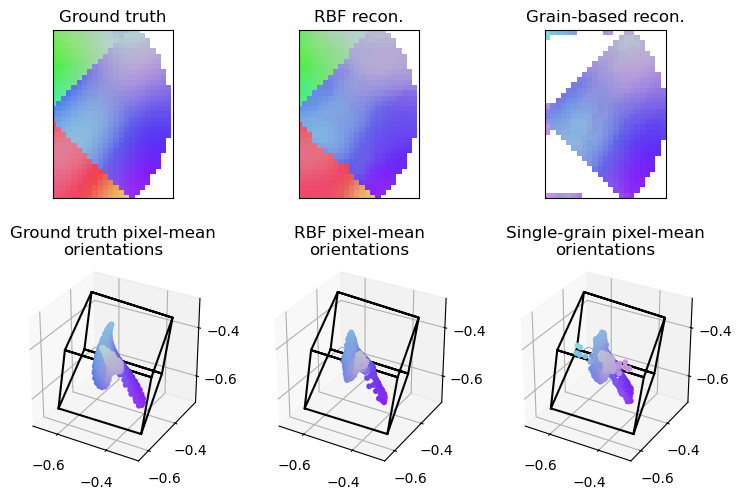
The typical IPF color mapping does not have high enough orientation contrast to see the difference, so we plot the \(\mathbf{r}\)-vector as RGB instead with a blown-up version of the typical OpenGL colormap for unit-vectors.
[52]:
fig = plt.figure(figsize = (9, 6))
gs = mpl.gridspec.GridSpec(2, 4, figure=fig, width_ratios = (1,1,1,0.1))

ax = fig.add_subplot(gs[0, 0])
gt_rotvec = (R.from_rotvec(gt_orientation_field.reshape((-1,3)))*grain_odf.average_orientation.inv())\
    .as_rotvec().reshape((*volume_shape, 3))
gt_rotvec_rgb = (gt_rotvec + grid_range) / 2 / grid_range
gt_rotvec_rgb[~gtmask, :] = 0
ax.imshow(gt_rotvec_rgb[:,0,:])
ax.set_xlim(bbox[4],bbox[5])
ax.set_ylim(bbox[1], bbox[0])
ax.set_title('Ground truth')
ax.set_xticks([]), ax.set_yticks([])

ax = fig.add_subplot(gs[0, 1])
RBF_rotvec = (R.from_rotvec(main_orientation_tomogram.reshape((-1,3)))*grain_odf.average_orientation.inv())\
    .as_rotvec().reshape((*volume_shape, 3))
RBF_rotvec_rgb = (RBF_rotvec + grid_range) / 2 / grid_range
RBF_rotvec_rgb[~grain_mask_full, :] = 0
ax.imshow(RBF_rotvec_rgb[:,0,:])
ax.set_xlim(bbox[4],bbox[5])
ax.set_ylim(bbox[1], bbox[0])
ax.set_title('RBF recon.')
ax.set_xticks([]), ax.set_yticks([])

ax = fig.add_subplot(gs[0, 2])
SG_rotvec = (R.from_rotvec(COM_orientation.reshape((-1,3)))*grain_odf.average_orientation.inv())\
    .as_rotvec().reshape((*grain_geometry.volume_shape, 3))
SG_rotvec_rgb = (SG_rotvec + grid_range) / 2 / grid_range
SG_rotvec_rgb[~grain_mask, :] = 0
ax.imshow(SG_rotvec_rgb[:,0,:], extent = (bbox[4],bbox[5],bbox[1], bbox[0]))
ax.set_title('Grain-based recon.')
ax.set_xticks([]), ax.set_yticks([])

ax = fig.add_subplot(gs[1, 1])
dev_from_gt = np.sqrt(np.sum((RBF_rotvec - gt_rotvec)**2, axis=-1))
dev_from_gt[~grain_mask_full] = 0
ax.imshow(dev_from_gt[:,0,:]*180/np.pi, vmin=0, vmax=3, cmap='jet')
ax.set_xlim(bbox[4],bbox[5])
ax.set_ylim(bbox[1], bbox[0])
ax.set_xticks([]), ax.set_yticks([])

ax = fig.add_subplot(gs[1, 2])
gt_rotvec_subsample = gt_rotvec[bbox[0]:bbox[1], bbox[2]:bbox[3], bbox[4]:bbox[5], :]
dev_from_gt_2 = np.sqrt(np.sum((SG_rotvec - gt_rotvec_subsample)**2, axis=-1))
dev_from_gt_2[~grain_mask] = 0
img = ax.imshow(dev_from_gt_2[:,0,:]*180/np.pi, extent=(bbox[4],bbox[5],bbox[1], bbox[0]), vmin=0, vmax=3, cmap='jet')
ax.set_xticks([]), ax.set_yticks([])

cax = fig.add_subplot(gs[1, 3])
cbar = fig.colorbar(img, cax=cax, label='Error')
cax.set_yticks([0, 1, 2, 3])
cax.set_yticklabels(['0°', '1°', '2°', '3°'])

ax = fig.add_subplot(gs[1, 0])
plt.hist(dev_from_gt[grain_mask_full]*180/np.pi, range = (0, 3), bins = 15, alpha = 0.7)
plt.hist(dev_from_gt_2[grain_mask]*180/np.pi, range = (0, 3), bins = 15, alpha = 0.7)
ax.set_xticks([0, 1, 2, 3])
ax.set_xticklabels(['0°', '1°', '2°', '3°'])
plt.legend(['RBF', 'Single grain'])
plt.show()
WARNING:Clipping input data to the valid range for imshow with RGB data ([0..1] for floats or [0..255] for integers). Got range [0.0..3.1362270062255315].
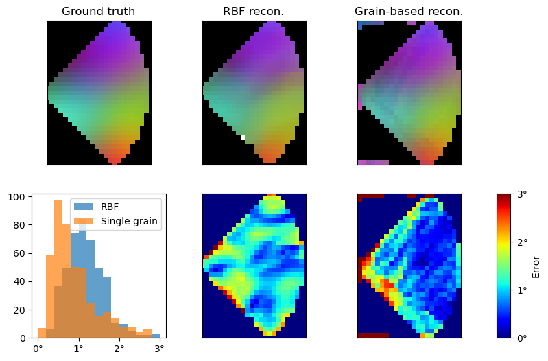
Figure caption: a) Ground truth intergranular misorientation(deviation from mean) in blown-up RGB colormap b) Reconstructed intergranular misorientation with RBF workflow and c) with single grain workflow. d) Histogram of orientation erros made with the two reconstructions and map of the same errors for e) RBF and f) Single grain.