Azimuthal Integration
The main reconstruction in texture tomography operates on azimuthally re-grouped diffraciton patterns. To create this azimuthally integrated data, we recommend using pyFAI because it is easy to use and is actively maintained.
When you have managed to open your detector files and have a working calibration file, the next step is to find a set of parameters for the radial integration:
A set of radial ranges covering the powder rings,
The number of azimuthal bins
Background subtraction.
Crystallography
Texture tomgraphy tries to fit the radially integrated intensities, which means you have to first index your powder rings and then prepare a set of \(2 \theta\) ranges that cover each diffraction ring.
When you know the crystal lattice, you can generate the lattice matrix and reciprocal lattice matrix using the ultility function in odftt.crystallography.crystal_families, the hkl-indicies should be given as a list of tuples, eg.:
hkl_list = [
    (1, 1, 1),
    (2, 2, 0),
    (3, 1, 1),
    (4, 0, 0),
]
This is the only occurence of Miller-indicies in the code. For the texture-funtions we use (often normalized) \(\mathbf{h}\)-vectors i.e. \(\mathbf{h}=\mathrm{B}[h, k, \ell]\), where \(\mathrm{B}\) is the reciprocal lattice matrix.
For monoclinic, rhombohedral, and hexagonal, there is an issue of how to choose the reciprocal lattice matrix. In principle any choice will do, but it is important that the \(\mathrm{B}\) matrix and the point group symmetry matrixes used for the texture functions live in the same coordinate system. SO you cannot use the upper-triangular form and for the monoclinic system, there is a strong preference to write the lattice matrix with the 2-fold symmetry aligned with the y axis while for the rotation groups I have written it down with the z-axis.
When the peaks have been identified, we need to choose integration regions to find the intensity. The most straight forward is to use bins of fixed width in \(2 \theta\) centered on each peak. If some peaks are significanlty overlapping, I ususally discard them.
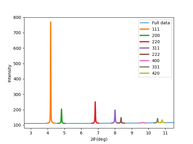
Radial bins created by a fixed width around each expected Bragg-peak position.
Azimuthal bins
The first parameter we need to choose which has an impact on the reconstruction workflow is the number of azimuthal bins. So far, my approach has been to try to match the azimuthal resolution with the scanning step in \(\omega\) (So if we have e.g. 100 sample rotations over 180°, I would use 200 azimuthal bins over 360°). This is because I like to have equal resolution but I have not tested the impact of this choice thoroughly.
When testing the reconstruciton workflow, it often makes sense to deliberately under-sample by binning the data (in both azimuth (\(\eta\)), sample rotation (\(\omega\)), and scanning y) to make the resontructions faster when figuing out the alignment and geometric parameters.
Background subtraction
Texture tomography fits to the integrated intensity of diffraciton features, so background subtraction is critical. In the easiest cases, the background is either constant or scales with the transmission of the sample. In such cases, the background from a no-sample measurement can be subtracted, potentially scaled by the transmission.
A more difficult case is when the background contains are large term of air-scattering, which comes from upstream of the sample. In this case, the sample shadows the scattering and the background on the detector depends on the sample position in a way that is different for different detector azimuths (\(\eta\)). If the data-quality is good and the diffraction peaks are well separated, we can do frame-by-frame background subtraction by selecting a region covering each peak and subtracting a linear background for each detector azimuth.
In general the reconstructions are quite noise tolerant, but leaving a large flat background does not work.
Transmission correction
For large samples, we need to correct for the transmission of x-rays through the sample. We do this approximately by normalizing the measured data with the transmission of the direct beam, which is ideally measured during the experiment using some sort of detector placed on the beamstop. If we did not measure the transmission during the experiment, we can instead model it. For dense single material samples, it suffices to create an outline of the sample, eg. by filtered back projection of the average scattering data, and use the projection of this outline to calculate transmission coefficients.
The most strongly absorbing samples we have worked with have transmission around 0.5.
Scaling factors
As we are only fitting the texture-factor, all other \(2\theta\) dependent factors in the integrated intensity have to be normalized out. These include the structure factor, Lorenz factor, the solid angle correction, Debye-Waller factor, and the polarization correction.
Aside from the polarization correction, which should be corrected for, the remaining factors can be calculated from the data directly. The usual texture tomography scan has quite good pole-figure coverage, so it is possible to calculate the normalization factors well, even from samples with strong macroscopic texture. Just remember to do the normalization after the transmission correction and background subtraction.
It is important to weight by the solid-angle coverage of each re-grouped data point. Otherwise the divergence of the Lorenz-factor at azimuths close to the tomographic axis can cause trouble if the sammple happens to have a strong feature there.
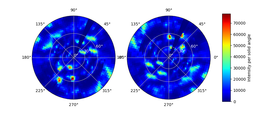
Typical pole figure coverage of a texture tomography scan.