Azimuthal integration workflow

This is a demonstration of how to create the azimuthally integrated data array using pyFAI.

You need to already have the following:

1. Detector images

2. pyFAI calibration file

3. Bad pixels mask

Then you need to manually find some parameters for the integration. Then you will need to make some batch-scipt to perform the integration on all the files and same the output. The last part I will not help you with.

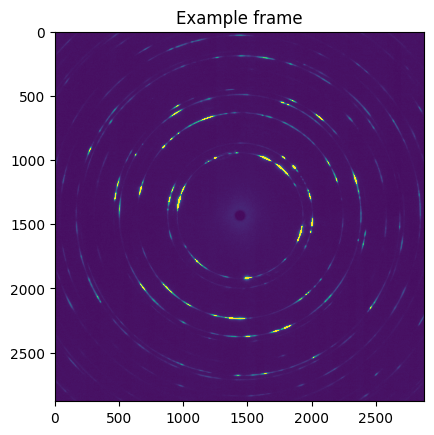
Let’s make sure that we can open the files and that they have data in them:

import fabio
import matplotlib.pyplot as plt
image_data = fabio.open('data/frame_123163.cbf').data
fig = plt.figure()
plt.imshow(image_data, vmax=300, vmin =100)
plt.title('Example frame')
fig.show()

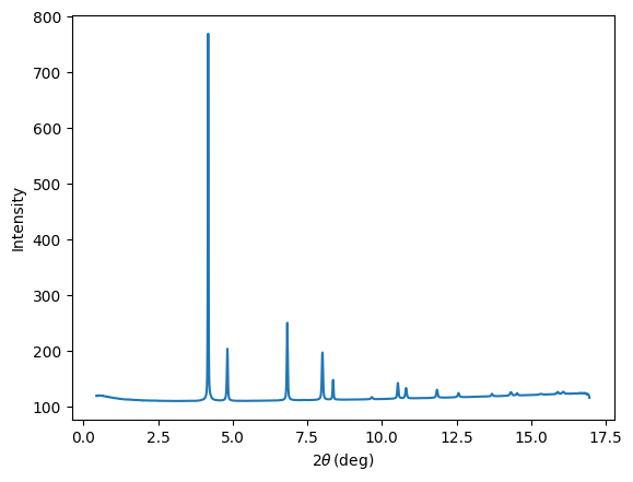
Now we set up a pyFAI.AzimuthalIntegrator-object and do a full azimuthal integration of the diffraction pattern. (called 1D integration in pyFAI)

import pyFAI
ai = pyFAI.load('data/online_lab6_calibration.poni')
mask = fabio.open('data/hot_pixels.edf').data + fabio.open('data/beamstop.edf').data
integration_args = {'npt':2000,'unit':'2th_deg','mask':mask}

tt_deg, intens = ai.integrate1d_ng(image_data, **integration_args)

fig = plt.figure()
plt.plot(tt_deg, intens)
plt.xlabel(r'$2\theta\,\text{(deg)}$')
plt.ylabel(r'Intensity')
fig.show()

WARNING:silx.opencl.common:Unable to import pyOpenCl. Please install it from: https://pypi.org/project/pyopencl

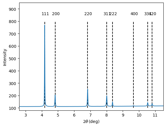
Now we calculate the expected position of the diffraction-peaks with standard x-ray crystallography:

import numpy as np
from odftomo.crystallography import cubic
A, B = cubic(a=3.98)
wavelength_ang = 0.16756

hkl_list = [(1, 1, 1),
            (2, 0, 0),
            (2, 2, 0),
            (3, 1, 1),
            (2, 2, 2),
            (4, 0, 0),
            (3, 3, 1),
            (4, 2, 0),]

def hkl_to_twotheta(hkl):
    return np.rad2deg(2*np.arcsin(np.linalg.norm(B @ hkl)/4/np.pi * wavelength_ang))

bragg_tt_deg_list = [hkl_to_twotheta(hkl) for hkl in hkl_list]

fig = plt.figure()
for hkl, bragg_twotheta_deg in zip(hkl_list, bragg_tt_deg_list):
    plt.plot([bragg_twotheta_deg]*2, [100, 800], 'k--')
    plt.text(bragg_twotheta_deg-0.2, 850, f'{hkl[0]}{hkl[1]}{hkl[2]}', color='k')
plt.plot(tt_deg, intens)

plt.xlabel(r'$2\theta\,\text{(deg)}$')
plt.ylabel(r'Intensity')
plt.xlim([2.6, 11.5])
plt.ylim(80, 950)
fig.show()

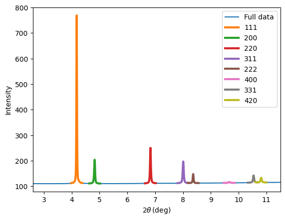
Next step is to define a set of ranges that cover the peaks. For this data, we have very well-separated peaks, so we can just pick a constant width.

fixed_width_deg = 0.4
tt_ranges = [(tt_deg-fixed_width_deg/2, tt_deg+fixed_width_deg/2) for tt_deg in bragg_tt_deg_list]

fig = plt.figure()

plt.plot(tt_deg, intens)
for tt_range in tt_ranges:
    peak_indicies = np.logical_and(tt_deg>=tt_range[0], tt_deg<tt_range[1])
    plt.plot(tt_deg[peak_indicies], intens[peak_indicies], linewidth=3)

plt.xlabel(r'$2\theta\,\text{(deg)}$')
plt.ylabel(r'Intensity')
plt.xlim([2.6, 11.5])
plt.ylim(80, 800)
leg = [f'{hkl[0]}{hkl[1]}{hkl[2]}' for hkl in hkl_list]
leg.insert(0, 'Full data')
plt.legend(leg)
plt.savefig('../img/radial_bin_widths.png')
fig.show()

Now we are ready to do azimuthal caking (called 2D-integration in pyFAI).

integration_args = {'npt_rad':2000, 'npt_azim':360, 'unit':'2th_deg',
                    'mask':mask, 'polarization_factor':0.95}
cake_data, tt_deg, azim_deg  = ai.integrate2d(image_data, **integration_args)
tt_stepsize = tt_deg[1] - tt_deg[0]
cake_imshow_extent = (tt_deg[0]-tt_stepsize/2, tt_deg[0-1]+tt_stepsize/2, 180, -180)

fig = plt.figure()
plt.imshow(cake_data,
           extent=cake_imshow_extent,
           vmin=100, vmax=500, aspect=0.03)

plt.title('Azimuthally caked data')
plt.xlabel(r'$2\theta\,\text{(deg)}$')
plt.ylabel(r'$\eta\,\text{(deg)}$')
fig.show()

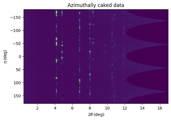
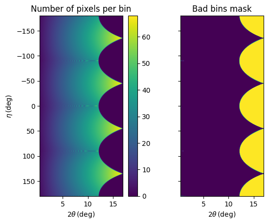
This is a nice flatpanel detector without gaps, but if you have gaps you need to mask them out in the texture tomography reconstruction later. This code snippet tries to do that in an automated manner by finding all bins that have less that half of the pixels expected for a bin at a given radius.

ones = np.ones(ai.get_shape())
integration_args_trick = {'npt_rad':2000, 'npt_azim':360, 'unit':'2th_deg',
                          'mask':mask, 'polarization_factor':None, 'correctSolidAngle':False}
_, _, _, variance = ai.integrate2d(ones, variance=ones, **integration_args_trick)
n_pix = 1/variance**2
n_pix[variance == 0] = 0

fig = plt.figure()

ax = plt.subplot(1,2,1)
plt.imshow(n_pix,
           extent=cake_imshow_extent,
           aspect=0.1)

plt.title('Number of pixels per bin')
plt.xlabel(r'$2\theta\,\text{(deg)}$')
plt.ylabel(r'$\eta\,\text{(deg)}$')
plt.colorbar()

n_pix[n_pix == 0]= np.nan
bins_mask = n_pix < 0.5 * np.nanmedian(n_pix, axis = 0)[np.newaxis, :]
bins_mask += np.isnan(n_pix)

ax = plt.subplot(1,2,2)
plt.imshow(bins_mask,
           extent=cake_imshow_extent,
           aspect=0.1)

plt.title('Bad bins mask')
plt.xlabel(r'$2\theta\,\text{(deg)}$')
ax.set_yticklabels([])
fig.show()

/tmp/ipykernel_3275806/327119571.py:5: RuntimeWarning: divide by zero encountered in divide
  n_pix = 1/variance**2

This data looks very clean, but there is a large flat background (either from air scattering or from dark-current). As the goal of texture tomography is to fit the intensities, background subtraction is critical.

In general background subtraction can be quite difficult. Here, we just make a polynomial fit to the part not containing any Bragg-peaks and interpolate into the part with the Bragg-peaks .

mean_data_radial = np.sum(~bins_mask*cake_data, axis = 0) / np.sum(~bins_mask, axis = 0)
peak_masks = [np.logical_and(tt_deg>=tt_range[0], tt_deg<tt_range[1]) for tt_range in tt_ranges]
any_peak_mask = np.sum(np.stack(peak_masks, axis = -1), axis = -1) > 0

mean_data_nopeaks = mean_data_radial[~any_peak_mask]
tt_nopeaks = tt_deg[~any_peak_mask]

bg_fit_coeffs = np.polyfit(tt_nopeaks[200:900], mean_data_nopeaks[200:900], 2)
bg = np.polyval(bg_fit_coeffs, tt_deg)

fig = plt.figure()
ax = plt.subplot(2,1,1)
plt.plot(tt_deg, mean_data_radial)
plt.plot(tt_deg, bg)
plt.legend(['Data', 'Background'])
plt.xlim(3, 13)
plt.ylim(108, 133)
plt.grid()

ax = plt.subplot(2,1,2)
plt.plot(tt_deg, (mean_data_radial- bg), color = 'C2')
plt.ylabel('Data - Background')
plt.xlim(3, 13)
plt.ylim(-3, 22)
plt.xlabel(r'$2\theta\,\text{(deg)}$')
plt.grid()
fig.show()

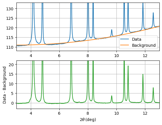
(Notice the nice little ferrite peaks!)

Now everything is finally ready to set up radial integration.

def process_one_frame(image_data):

    cake_data, _, _  = ai.integrate2d(image_data, **integration_args)
    cake_data = cake_data - bg[np.newaxis, :]
    output_data = []
    for peak_mask in peak_masks:
        this_peak_data = np.sum(cake_data[:, peak_mask], axis = -1)
        output_data.append(this_peak_data)

    return np.stack(output_data, axis = -1)

integrated_data = process_one_frame(image_data)

fig = plt.figure()
for hkl_index, hkl in enumerate(hkl_list):

    if hkl_index <= 3:
        plt.plot(azim_deg, integrated_data[:, hkl_index] + hkl_index * 3e4)
        plt.text(150, hkl_index * 3e4 + 6e3, f'{hkl[0]}{hkl[1]}{hkl[2]}', color = f'C{hkl_index}')
    elif hkl_index > 3:
        plt.plot(azim_deg, integrated_data[:, hkl_index]*10 + hkl_index * 3e4)
        plt.text(100, hkl_index * 3e4 + 6e3, f'{hkl[0]}{hkl[1]}{hkl[2]} (times 10)', color = f'C{hkl_index}')

plt.yticks( np.arange(len(hkl_list))*3e4, labels = [])
plt.grid()
plt.xlim(-180, 180)
plt.ylim(-1e4, 2.3e5)
plt.xlabel(r'$\eta\,\text{(deg)}$')
plt.show()

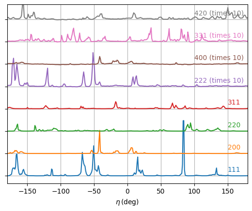
The parallel reflections (111 and 222, and 200 and 400) are strongly correlated but not identical because of the \(\Delta 2\theta\) offset in direction.