Centroid orientations and clustering algorithms

Tasks such as computing the mean orientation and clustering orientations data is more difficult than one would expect because of the complicated topology of crystal-orientation spaces, which means that the typical coordinates used for orientations: Euler angles, rotation vectors, and quaternions, have periodic boundary conditions.

These periodic boundary conditions mean that the standard approach for computing the centroid, the mean, does not work. The figure below tries to demonstrate this with a simple 2D toy-problem:

# Draw a pointcloud from a gaussian distributions
import numpy as np

def cluster_of_points(N, mean, cov):
    points = np.random.multivariate_normal(mean, cov, N).T
    points = points%1  # Toroidial boundary conditions
    return points

mean_1 = np.array([0.95, 0.2])
cov_1 = np.array([[0.015, 0.004], [0.004, 0.004]])
cluster_1 = cluster_of_points(60, mean_1, cov_1)

import matplotlib.pyplot as plt

# Make somu utility functions for plotting
angles = np.linspace(0, 2*np.pi, 101)
def make_ellipse(mean, cov, N_sigmas):
    eivals, eigvecs = np.linalg.eig(cov)
    vecs = (np.cos(angles)*np.sqrt(eivals[0]))[np.newaxis, :]*eigvecs[:,0,np.newaxis]*N_sigmas\
            + (np.sin(angles)*np.sqrt(eivals[1]))[np.newaxis, :]*eigvecs[:,1,np.newaxis]*N_sigmas\
            + mean[:, np.newaxis]
    return vecs

angles_1 = np.linspace(0, np.pi, 100)
angles_2 = np.linspace(0, 2*np.pi, 100)
def make_ellipsoid(mean, cov, N_sigmas):
    eivals, eigvecs = np.linalg.eig(cov)
    g = R.from_rotvec(mean)

    v1 = np.cos(angles_1)[:, np.newaxis]
    v2 = np.sin(angles_1)[:, np.newaxis]*np.cos(angles_2)[np.newaxis, :]
    v3 = np.sin(angles_1)[:, np.newaxis]*np.sin(angles_2)[np.newaxis, :]

    vecs = v1[np.newaxis, :, :]*eigvecs[:,0,np.newaxis, np.newaxis]*N_sigmas*np.sqrt(eivals[0])\
          +v2[np.newaxis, :, :]*eigvecs[:,1,np.newaxis, np.newaxis]*N_sigmas*np.sqrt(eivals[1])\
          +v3[np.newaxis, :, :]*eigvecs[:,2,np.newaxis, np.newaxis]*N_sigmas*np.sqrt(eivals[2])\

    rots = R.from_rotvec(vecs.reshape((3,-1)).T)
    rots = rots * g
    vecs = rots.as_rotvec().T.reshape((3,100,100))
    return vecs

def plot_box(ax):
    ax.plot([0,0], [0,1], 'b')
    ax.plot([1,1], [0,1], 'b')
    ax.plot([0,1], [0,0], 'r')
    ax.plot([0,1], [1,1], 'r')
    ax.set_aspect('equal', 'box')
    ax.axis('off')
    ax.set_xlim(-0.0, 1.0)
    ax.set_xlabel(r'$x_1$')
    ax.set_ylim(-0.0, 1.0)
    ax.set_ylabel(r'$x_2$')

# Make the plot
fig = plt.figure(figsize = (5, 5))
ax1 = plt.subplot(1,1,1)
scatt = ax1.scatter(*cluster_1, c='k', s=5 , alpha=1)
vecs = make_ellipse(mean_1, cov_1, 1)
elips = plt.plot(mean_1[0], mean_1[1], 'x', markersize=13, markeredgewidth=5, color='C0')
ax1.plot(vecs[0], vecs[1], color = 'C0')
vecs = make_ellipse(mean_1, cov_1, 2)
ax1.plot(vecs[0], vecs[1], '--',color = 'C0')
vecs = make_ellipse(mean_1-np.array([1,0]), cov_1, 1)
ax1.plot(vecs[0], vecs[1], color = 'C0')
vecs = make_ellipse(mean_1-np.array([1,0]), cov_1, 2)
ax1.plot(vecs[0], vecs[1], '--',color = 'C0')
plot_box(ax1)

mean = np.mean(cluster_1, axis=1)
mean_x = plt.plot(mean[0], mean[1], 'x', markersize=13, markeredgewidth=5, color='C1')
plt.legend([elips[0], scatt, mean_x[0]], ['Distribution centroid', 'Sample', 'Sample mean'],)
plt.show()

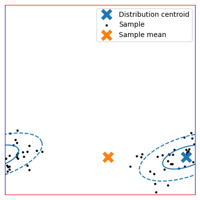
We draw a set of points from a 2D Gaussian distribution, then we put the data in a 1-by-1 box with toroidal boundary conditions such that part of the dataset appears on the other side of the domain.

This in turn means that the coordinate-wise average does not give a good estimate of the centroid position illustrated by the orange cross.

In this python package, we have implemented two kinds of algorithms to overcome this issue.

The notebook is split in two parts:

1. Iterative methods

2. Embedding methods

1. Iterative methods

Since orientation space is a Lie group, it is locally similar to Eucluidian space which means that if the cluster is small enough, the coordinate wise mean is a good estimate of the centroid when using apropriate coordinates. 3D rotation-vectors are one such good choice of coordinates for clusters close to the identity rotation, \(e\).

We can shift orientations towards \(e\) by composing with an estimate of the inverse centroid orientation, so the idea is to use the mean in rotation vector space as a rough estimate of the true centroid orientation and use this estimate to shift the data towards \(e\). Then repeat until convergence.

Let’s draw a random sample and see how this iterative algorithm performs.

from scipy.spatial.transform import Rotation as R
from odftomo.texture import point_groups, grids

# Utility functions to draw random crystal orientations
def cast_rots_tofundamental(rots, sym_group = point_groups.trivial):
    min_norm = np.pi*np.ones(len(rots))
    min_rotvecs = np.zeros( (len(rots),3) )
    for index, S in enumerate(sym_group):
        rot_rot = rots * S
        norm = rot_rot.magnitude()
        where = norm < min_norm
        min_norm[where] = norm[where]
        min_rotvecs[where,:] = rot_rot.as_rotvec()[where,:]
    return R.from_rotvec(min_rotvecs)

def draw_rotations(N, g_mean, sigma_deg, prolate_direction=np.array([0,0,1])):
    # Draw random quarternions at identity aligned with J_x
    sigma_rad = sigma_deg*np.pi/180
    random_quat = np.random.multivariate_normal(np.array([0, 0, 0, 1]),
                                                 np.diag(((sigma_rad/3)**2/np.pi, (sigma_rad/3)**2/np.pi, sigma_rad**2/np.pi, 0)),
                                                 size=(N),
                                                 check_valid='warn',
                                                 tol=1e-8)
    random_quat = random_quat / np.linalg.norm(random_quat, axis = 1)[:, np.newaxis]
    random_ori = R.from_quat(random_quat)
    # Rotate random sample
    R1 = R.from_euler('yz', [np.arccos(prolate_direction[2]), np.arctan2(prolate_direction[1], prolate_direction[0])])
    ori =  R1 * random_ori * R1.inv() *g_mean
    return ori

# Draw a random sample of orientations
distr_cen = R.from_rotvec([0.8, -0.5, 0.35])
distr_prolate_dir = R.from_euler('ZY', [0, 0]).apply([0, 0, 1])
sigma_deg = 10
g_cluster = cast_rots_tofundamental(draw_rotations(100, distr_cen, sigma_deg , distr_prolate_dir), point_groups.hexagonal)
rotvecs =  g_cluster.as_rotvec()

from odftomo.analysis.segmentation import blob_finder
# Find mean oprientation with iterative algorithm
component = blob_finder(np.ones(len(g_cluster)), 1, 180, g_cluster, point_groups.hexagonal)[0]
rv = component.COM_ori.as_rotvec()

/home/madsac/miniconda3/envs/odftt/lib/python3.13/site-packages/odftomo/analysis/grid_tools.py:113: RuntimeWarning: invalid value encountered in arccos
  dist_this = np.arccos(2*np.abs(np.einsum('ik,k->i',

from odftomo import plot_tools

# Build the plot
plt.figure(figsize = (9,8))
ax = plt.subplot(1,1,1, projection = '3d',computed_zorder=False)
scatt = ax.scatter(rotvecs[:,0],rotvecs[:,1],rotvecs[:,2], s=2, alpha=1.0, c='k') # Scatter plot of sample
# Elipsoid at sigma=2 level
sigma_rad = sigma_deg*np.pi/180
mat = R.from_euler('ZY', [0, 0]).as_matrix()
distr_cov = 4 * mat @ np.diag(((sigma_rad/3)**2/np.pi, (sigma_rad/3)**2/np.pi, sigma_rad**2/np.pi)) @ mat.T
ellipsoid_vecs = make_ellipsoid(distr_cen.as_rotvec(), distr_cov, 2)
elips = ax.plot_wireframe(ellipsoid_vecs[0], ellipsoid_vecs[1], ellipsoid_vecs[2],
                          rstride=10, cstride=10, alpha=1.0, zorder=1, linewidth=0.5, color='C0')
# Mean rotvec
rotvec_mean = np.mean(rotvecs, axis=0)
mean_x = plt.plot(rotvec_mean[0], rotvec_mean[1], rotvec_mean[2], 'x', markersize=13, markeredgewidth=5, color='C1')

it_x = plt.plot(rv[0], rv[1], rv[2], 'x', markersize=13, markeredgewidth=5, color='C2')  # Iterative solution point

plt.legend([elips, scatt, mean_x[0], it_x[0]], ['Distribution', 'Sample', 'Sample mean', 'Iterative'],)
plot_tools.plot_asym_zone_outline(ax, 'hexagonal')
ax.axis('scaled')
ax.view_init(azim = 0, elev = 3)
plt.show()

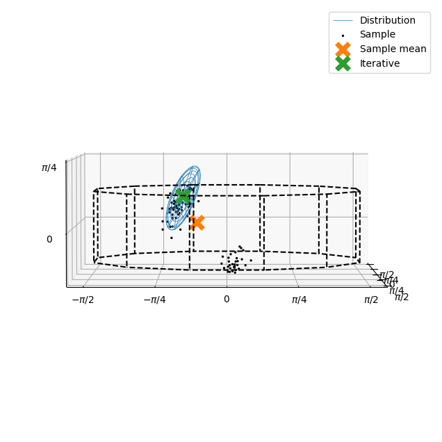
A part of the orientations sample crosses the boudary of the asymmetric zone and appears in the other side of the asymmetric zone. This causes the mean in rotvec coordinates to give a bad estimate of the distribution centroid.

The iterative method does better and finds a point inside the pointcloud.

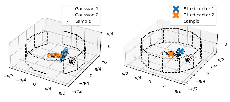
The main use of the clustering algorthm is to identify texture components (grains) in individual pixels of RBF reconstructions. This means the algorithm also needs to be able to handle mutiple components in a voxel.

The simple solution we have gone with for now is to add a few extra parameters to the algorithm, which are: (1) a max radius of a texture component and (2) a minimum number of samples for a component, to avoid noisy data points to be classified as texture components.

To illustrate, we draw a mixture of two Gaussians and recover the clusters:

# Draw from a second Bingham distribution
distr_cen_2 = R.from_rotvec([0.0, -0.1, -0.20])
distr_prolate_dir_2 = R.from_euler('ZY', [0.5, np.pi/2]).apply([0, 0, 1])
g_cluster_2 = cast_rots_tofundamental(draw_rotations(50, distr_cen_2, sigma_deg , distr_prolate_dir_2), point_groups.hexagonal)
rotvecs_2 =  g_cluster_2.as_rotvec()

# Combine the two samples
combined_rotvec = np.concatenate([rotvecs, rotvecs_2], axis=0)
g_cluster_combined = R.from_rotvec(combined_rotvec)

# Do the clsutering
max_radius_degrees = 20
min_number_points = 10
components = blob_finder(np.ones(len(g_cluster_combined)), min_number_points,
                        max_radius_degrees, g_cluster_combined, point_groups.hexagonal)

#Build the plot
plt.figure(figsize = (9,6))

ax = plt.subplot(1,2,1, projection = '3d',computed_zorder=False)
scatt = ax.scatter(combined_rotvec[:,0],combined_rotvec[:,1],combined_rotvec[:,2], s=2, alpha=1.0, c='k')  # Random sample
# Draw distribution outline first gaussian
sigma_rad = sigma_deg*np.pi/180
mat = R.from_euler('ZY', [0, 0]).as_matrix()
distr_cov = 4 * mat @ np.diag(((sigma_rad/3)**2/np.pi, (sigma_rad/3)**2/np.pi, sigma_rad**2/np.pi)) @ mat.T
ellipsoid_vecs = make_ellipsoid(distr_cen.as_rotvec(), distr_cov, 2)
elips = ax.plot_wireframe(ellipsoid_vecs[0], ellipsoid_vecs[1], ellipsoid_vecs[2],
                          rstride=10, cstride=10, alpha=1.0, zorder=1, linewidth=0.5, color='C0')
# Draw distribution outline second gaussian
sigma_rad = sigma_deg*np.pi/180
mat = R.from_euler('ZY', [0.5, np.pi/2]).as_matrix()
distr_cov = 4 * mat @ np.diag(((sigma_rad/3)**2/np.pi, (sigma_rad/3)**2/np.pi, sigma_rad**2/np.pi)) @ mat.T
ellipsoid_vecs = make_ellipsoid(distr_cen_2.as_rotvec(), distr_cov, 2)
elips2 = ax.plot_wireframe(ellipsoid_vecs[0], ellipsoid_vecs[1], ellipsoid_vecs[2],
                          rstride=10, cstride=10, alpha=1.0, zorder=1, linewidth=0.5, color='C1')
plt.legend([elips, elips2, scatt], ['Gaussian 1', 'Gaussian 2', 'Sample'],)
plot_tools.plot_asym_zone_outline(ax, 'hexagonal')
ax.axis('scaled')


ax = plt.subplot(1,2,2, projection = '3d',computed_zorder=False)
scatt = ax.scatter(combined_rotvec[:,0],combined_rotvec[:,1],combined_rotvec[:,2], s=2, alpha=1.0, c='k')
handles = []
for component, color in zip(components, ['C0', 'C1']):
    rv = component.COM_ori.as_rotvec()
    handle = plt.plot(rv[0], rv[1], rv[2], 'x', markersize=13, markeredgewidth=5, color=color)[0]
    handles.append(handle)
plt.legend([*handles, scatt], ['Fitted center 1', 'Fitted center 2', 'Sample'],)
plot_tools.plot_asym_zone_outline(ax, 'hexagonal')
ax.axis('scaled')
plt.show()

2. Embedding methods

I mainly use the embedding methods to compute the main orientation from GSH reconstructions. To explain the idea, we return to the 2D example from the introduction.

The 2D square with periodic boundary conditions can be embedded in 3D on the surface of a torus. In these coordinates, the boundary conditions are naturally expressed and the mean in 3D will now lie close to the point cloud. There is new problem however; the mean no longer lies on the 2D manifold of the torus, which mean it needs to be projected onto the manifold.

The figure below illustrates the process:

# Utility scipts with geometry of torus
R = 1; r = 0.5
def map_to_torus(ang1, ang2):

    vector = np.stack([
        np.sin(ang1*np.pi*2) * r,
        (np.cos(ang1*np.pi*2) * r + R)*np.cos(ang2*np.pi*2),
        (np.cos(ang1*np.pi*2) * r + R)*np.sin(ang2*np.pi*2),
    ], axis=0)
    return vector

def project_to_torus(vector):

    ang2 = np.arctan2(vector[2], vector[1])
    d = np.sqrt(vector[1]**2 + vector[2]**2)
    ang1 = np.arctan2(vector[0], d-R)
    return np.array([ang1/np.pi/2, ang2/np.pi/2])%1

def tangent_vectors(ang1, ang2):

    tv1 = np.array([
        np.cos(ang1*np.pi*2) * r,
        -np.sin(ang1*np.pi*2)*np.cos(ang2*np.pi*2)*r,
        -np.sin(ang1*np.pi*2)*np.sin(ang2*np.pi*2)*r,
    ])

    tv2 = np.array([
        0,
        -(np.cos(ang1*np.pi*2) * r + R)*np.sin(ang2*np.pi*2),
        (np.cos(ang1*np.pi*2) * r + R)*np.cos(ang2*np.pi*2),
    ])

    return np.stack([tv1, tv2], axis = -1)*np.pi*2

# Draw a 2D point cloud
mean_1 = np.array([0.95, 0.12])
cov_1 = np.array([[0.015, 0.004], [0.004, 0.004]])
cluster_1 = cluster_of_points(60, mean_1, cov_1)%1

# Embed in 3D
data_3d = map_to_torus(cluster_1[0], cluster_1[1])

# Do statistics in 3D
mean_3d = np.mean(data_3d, axis=1)
cov_3d = data_3d @ data_3d.T/data_3d.shape[1] - np.outer(mean_3d,mean_3d)

# Map back to 2D
mean_proj = project_to_torus(mean_3d)

M = tangent_vectors(*mean_proj)
norms = np.diag(np.linalg.norm(M, axis = 0)**(-2))
M = M @ norms
cov_2d = M.T @ cov_3d @ M

# Build a large plot
fig = plt.figure(figsize = (9, 9))

# 2D data
ax1 = plt.subplot(2,2,1)
scatt = ax1.scatter(*cluster_1, c='k', s=5 , alpha=1)
vecs = make_ellipse(mean_1, cov_1, 1)
elips = plt.plot(mean_1[0], mean_1[1], 'x', markersize=13, markeredgewidth=5, color='C0')
ax1.plot(vecs[0], vecs[1], color = 'C0')
vecs = make_ellipse(mean_1, cov_1, 2)
ax1.plot(vecs[0], vecs[1], '--',color = 'C0')
vecs = make_ellipse(mean_1-np.array([1,0]), cov_1, 1)
ax1.plot(vecs[0], vecs[1], color = 'C0')
vecs = make_ellipse(mean_1-np.array([1,0]), cov_1, 2)
ax1.plot(vecs[0], vecs[1], '--',color = 'C0')
plot_box(ax1)
mean = np.mean(cluster_1, axis=1)
mean_x = plt.plot(mean[0], mean[1], 'x', markersize=13, markeredgewidth=5, color='C1')
plt.legend([elips[0], scatt, mean_x[0]], ['Distribution centroid', 'Sample', 'Sample mean'],)
plt.title('Original distribution')

# Data on torus
ax = plt.subplot(2,2,2, projection='3d', computed_zorder=False)
plt.title('Embedded data')
ax.scatter(data_3d[0], data_3d[1], data_3d[2], alpha=1, color='k')
# Make the torus outline
wireframe_1 = np.linspace(0, 1, 160)
wireframe_2 = np.linspace(0, 1, 200)
wireframe_1, wireframe_2 = np.meshgrid(wireframe_1, wireframe_2)
wireframe_3d = map_to_torus(wireframe_1, wireframe_2)
ax.plot_wireframe(wireframe_3d[0], wireframe_3d[1], wireframe_3d[2], color = [0.4,0.4,0.4],
                  rstride=20, cstride=10,zorder=0, linewidth = 0.5)
# PLot the distribution on the torus
centroid_3d = map_to_torus(*mean_1)
elips = plt.plot(*centroid_3d, 'x', markersize=13, markeredgewidth=5, color='C0')
vecs_3d = map_to_torus(*make_ellipse(mean_1, cov_1, 1))
ax.plot(vecs_3d[0], vecs_3d[1], vecs_3d[2], '-', color = 'C0', linewidth = 2)
vecs_3d = map_to_torus(*make_ellipse(mean_1, cov_1, 2))
ax.plot(vecs_3d[0], vecs_3d[1], vecs_3d[2], '--', color = 'C0', linewidth = 2)
ax.axis('scaled')
ax.view_init(azim = 0, elev = 45+90)

# Statistics in 3D
ax = plt.subplot(2,2,3, projection='3d')
ax.scatter(data_3d[0], data_3d[1], data_3d[2], alpha=0.3, color='k', s = 2)
# Torus outline
wireframe_1 = np.linspace(0, 1, 160)
wireframe_2 = np.linspace(0, 0.25, 50)
wireframe_1, wireframe_2 = np.meshgrid(wireframe_1, wireframe_2)
wireframe_3d = map_to_torus(wireframe_1, wireframe_2)
ax.plot_wireframe(wireframe_3d[0], wireframe_3d[1], wireframe_3d[2], color = [0.4,0.4,0.4],
                  rstride=20, cstride=10,zorder=0, linewidth = 0.5)
# Mean in 3D
mean_embedded_dot = plt.plot(*mean_3d, '.', markersize=13, markeredgewidth=5, color='C2')
plt.plot(*np.stack([mean_proj, mean_proj], axis=1) , '--', color='C2')
mean_proj_emb = map_to_torus(*mean_proj)
mean_projected_x = plt.plot(*mean_proj_emb, 'x', markersize=13, markeredgewidth=5, color='C2')
# Coordinate lines of projected mean to help the eye
wireframe_1 = np.linspace(0, 1, 160)
wireframe_2 = np.linspace(0, 0.25, 50)
vecs_3d = map_to_torus(wireframe_1, mean_proj[1]*np.ones(len(wireframe_1)))
ax.plot(vecs_3d[0], vecs_3d[1], vecs_3d[2], '--', color = 'C2', linewidth = 1)
vecs_3d = map_to_torus(mean_proj[0]*np.ones(len(wireframe_2)), wireframe_2)
ax.plot(vecs_3d[0], vecs_3d[1], vecs_3d[2], '--', color = 'C2', linewidth = 1)

ax.view_init(azim = 0, elev = 45+90)
ax.set_ylim(0, 1.5)
ax.set_zlim(0, 1.5)
plt.legend([mean_embedded_dot[0], mean_projected_x[0]], ['Embedded mean', 'Embedded mean projected'],loc='lower center')

# Projected onto 2D
ax1 = plt.subplot(2,2,4)
scatt = ax1.scatter(*cluster_1, c='k', s=5 , alpha=1)
vecs = make_ellipse(mean_proj, cov_2d, 1)
elips = plt.plot(mean_proj[0], mean_proj[1], 'x', markersize=13, markeredgewidth=5, color='C2')
ax1.plot(vecs[0], vecs[1], color = 'C2')
vecs = make_ellipse(mean_proj, cov_2d, 2)
ax1.plot(vecs[0], vecs[1], '--',color = 'C2')
vecs = make_ellipse(mean_proj-np.array([1,0]), cov_2d, 1)
ax1.plot(vecs[0], vecs[1], color = 'C2')
vecs = make_ellipse(mean_proj-np.array([1,0]), cov_2d, 2)
ax1.plot(vecs[0], vecs[1], '--',color = 'C2')
plot_box(ax1)
plt.title('Fitted distribution')
plt.show()

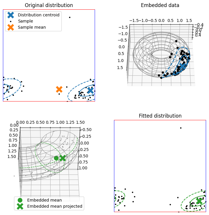
Figure caption: Illustration of embedding approach using toy-problem. a) Data is sampled in the 2D domain with periodic boudary conditions leading to problems with using the mean as a centroid estimate. b) By embedidng the data on a torus, the periodic boudary conditions disappear. c) The 3D mean can be computed and projected onto the torus, yealding a good estimate of the centroid position. d) The 3D covariance can also be projected into the 2D space giving an estimate of the original covariance of the distribution.

The main objective now is to find some higher-dimensional embedding where the boundary conditions are naturally expressed. Our suggestion is to use coefficients of low-order symmetrized spherical surface harmonics.

Spherical harmonics are equivalent to certain tensors, which have previously been used for this purpose [Arnold et al., Hielscher and Lippert] but the basis of real spherical harmonics coefficients is convenient because it is a conventional, low dimensional basis for the tensor spaces that does not contain the rotationally invariant subspaces and separates the different orders (irreducible representations) completely.

Furthermore, it is very easy to generate the embeddings and tangent vectors using Wigner’s matrices \(\mathrm{D}^\ell(g)\in \mathbb{R}^{(2\ell+1)\times(2\ell+1)}\) and the generators of the invariant representations \(J^\ell_{\alpha}\in \mathbb{R}^{(2\ell+1)\times(2\ell+1)}\) for \(\alpha \in {x,y,z}\). The embeddings themselves are of dimension \(2\ell+1\).

The goal is to find some coefficient vector \(\mathbf{h}\) which is symmetric under the lattice symmetry point group, \(S\):

\[\mathrm{D}^\ell(s)\mathbf{h} = \mathbf{h}\text{ for all }s\in S\]

Then the embedded orientations are generated simply by

\[\mathbf{h}(g) = \mathrm{D}^\ell(g)\mathbf{h}\]

The embedding approach then implies a distance function between orientations:

\[d(g_1, g_1) = \left|\left|\mathrm{D}^\ell(g_1)\mathbf{h}-\mathrm{D}^\ell(g_2)\mathbf{h}\right|\right|_2\]

This construction along with the unitarity property of the Wigner matrices ensures a number of symmetry properties but it does not ensure that rotations about different crystal axis by the same angle has the same norm. The best we can do is to pick a coefficient vector \(\mathbf{h}\) such that the implied norm is locally isometric, that is that all small rotations have the same norm.

For the cubic point group, the first harmonic which has the apropriate symmetry is at order \(\ell = 4\) and leads to a locally isometric norm. It is equivalent to the embdding used in the work cited above, but in this basis it is 9-dimensional instead of 15 and 14 in the bases used by Arnold and Hielscher respectively.

For hexagonal symmetry the first harmonic is at order \(\ell=6\) but at this order there is an extra degree of freedom for its construction. Any linear combination of \(Y_6^0\) and \(Y_6^6\), except with \(h_6=0\), has the right symmetry. Numerically we find that there is only one linear combination which achieves local isometry (apart for arbitrary sign and normalization):

from odftomo.spharm.spharm_tools import make_generators

ell = 6
J_alpha_list = make_generators(ell)
h_0_list = np.linspace(0,1,100)
v1 = []; v2 = []; v3 = []
for h_0 in h_0_list:
    h_6 = np.sqrt(1-h_0**2)
    h = np.array([0,0,0,0,0,0,h_0,0,0,0,0,0,h_6])
    tangent_vectors = np.stack([J_alpha @ h for J_alpha in J_alpha_list])
    n= np.linalg.norm(tangent_vectors, axis = 1)
    v1.append(n[0])
    v2.append(n[1])
    v3.append(n[2])

plt.plot(h_0_list, v1)
plt.plot(h_0_list, v2)
plt.plot(h_0_list, v3)

plt.xlabel(r'$h_0 / \sqrt{h_0^2 + h_6^2}$')
plt.ylabel(r'$\mathrm{J}_\alpha \mathbf{h}$')
plt.legend([r'$||J_x\mathbf{h}||$', '$||J_y\mathbf{h}||$', '$||J_z\mathbf{h}||$'])
plt.show()

<>:22: SyntaxWarning: invalid escape sequence '\m'
<>:22: SyntaxWarning: invalid escape sequence '\m'
<>:22: SyntaxWarning: invalid escape sequence '\m'
<>:22: SyntaxWarning: invalid escape sequence '\m'
/tmp/ipykernel_47031/161275513.py:22: SyntaxWarning: invalid escape sequence '\m'
  plt.legend([r'$||J_x\mathbf{h}||$', '$||J_y\mathbf{h}||$', '$||J_z\mathbf{h}||$'])
/tmp/ipykernel_47031/161275513.py:22: SyntaxWarning: invalid escape sequence '\m'
  plt.legend([r'$||J_x\mathbf{h}||$', '$||J_y\mathbf{h}||$', '$||J_z\mathbf{h}||$'])

INFO:Setting the number of threads to 8. If your physical cores are fewer than this number, you may want to use numba.set_num_threads(n), and os.environ["OPENBLAS_NUM_THREADS"] = f"{n}" to set the number of threads to the number of physical cores n.
INFO:Setting numba log level to WARNING.

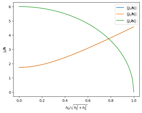
In the mumott phase and normalization convention this harmonic has the coefficients \(h_0 = \sqrt{11/18}\) and \(h_6 = \sqrt{7/18}\).

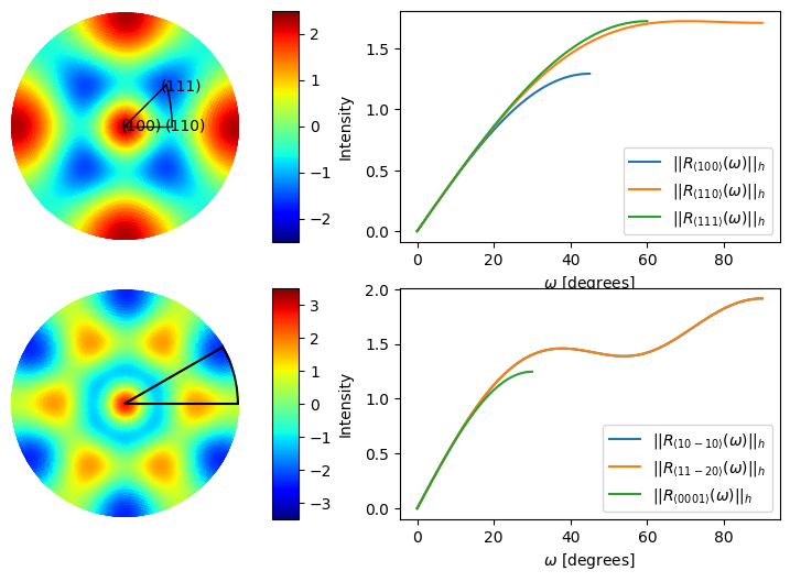
Unfortunately, for all the other point groups, it turns out to be more difficult to find appropriate coefficient vectors. For example trying to do the same procedure we did for hexagonal with tetragonal symmetry, we would recover the cubic symmetric harmonic which cannot be used as it has too high symmetry.

Hielscher and Lippert overcomes this issue by constructing embeddings that live in product spaces of several tensor space, and such an approach would probably work (I could just copy their solutions for example) but I have not gone through implementing it as I am mainly interested in cubic and hexagonal (metal) samples anyways.

The two embeddings and the implied norms of rotations about special axes are plotted below:

import matplotlib.gridspec as gridspec
from odftomo.analysis.harmonics_fitting import HarmonicFitter, MeanOrientationFinderGSH, compute_cluster_statistics, embedding_harmonics
from odftomo import plot_tools
from odftomo.texture import point_groups, grids, odfs
from scipy.spatial.transform import Rotation as R
from odftomo.spharm.spharm_tools import rotate_single_ell, map_single_l

fig = plt.figure(figsize = (9,6))
gs = gridspec.GridSpec(2, 4, figure=fig, width_ratios = [0.6,0.07, 0.09,1.0])
########### cubic ##################
h = embedding_harmonics['cubic'][0].coefficients
ell = embedding_harmonics['cubic'][0].ell

ax1 = fig.add_subplot(gs[0, 3])
axis = np.array([1,0,0])
angles = np.linspace(0, np.pi/4, 100)
g = R.from_rotvec(axis[np.newaxis, :] * angles[:, np.newaxis])
harmnorm = np.linalg.norm(h[np.newaxis, :] - rotate_single_ell(g, h, ell), axis = 1)
ax1.plot(angles * 180/np.pi, harmnorm)
axis = np.array([1,1,0])/np.sqrt(2)
angles = np.linspace(0, np.pi/2, 100)
g = R.from_rotvec(axis[np.newaxis, :] * angles[:, np.newaxis])
harmnorm = np.linalg.norm(h[np.newaxis, :] - rotate_single_ell(g, h, ell), axis = 1)
ax1.plot(angles * 180/np.pi, harmnorm)
axis = np.array([1,1,1])/np.sqrt(3)
angles = np.linspace(0, np.pi/3, 100)
g = R.from_rotvec(axis[np.newaxis, :] * angles[:, np.newaxis])
harmnorm = np.linalg.norm(h[np.newaxis, :] - rotate_single_ell(g, h, ell), axis = 1)
ax1.plot(angles * 180/np.pi, harmnorm)
plt.legend([r'$||R_{\langle 100 \rangle}(\omega)||_h$', r'$||R_{\langle 110 \rangle}(\omega)||_h$', r'$||R_{\langle 111 \rangle}(\omega)||_h$'])
plt.xlabel(r'$\omega$ [degrees]')

ax2 = fig.add_subplot(gs[0, 0], polar=True)
map_theta = np.linspace(0, np.pi/2, 91)
map_phi = np.linspace(0, np.pi*2, 361)
map_intens = map_single_l(ell, h, map_theta, map_phi)
img = ax2.pcolormesh(map_phi, np.tan(map_theta/2), map_intens, edgecolors = 'face', rasterized = True, cmap = 'jet', vmin = -2.5, vmax = 2.5)
cax =  fig.add_subplot(gs[0, 1])
fig.colorbar(img, cax=cax, label = 'Intensity')
plot_tools.polefigure.plot_cubic_asym_outline(ax2)
ax2.axis('off')

########### hexagonal ##################
h = embedding_harmonics['hexagonal'][0].coefficients
ell = embedding_harmonics['hexagonal'][0].ell

ax1 = fig.add_subplot(gs[1, 3])
axis = np.array([1,0,0])
angles = np.linspace(0, np.pi/2, 100)
g = R.from_rotvec(axis[np.newaxis, :] * angles[:, np.newaxis])
harmnorm = np.linalg.norm(h[np.newaxis, :] - rotate_single_ell(g, h, ell), axis = 1)
ax1.plot(angles * 180/np.pi, harmnorm)
axis = np.array([np.cos(np.pi/3),np.sin(np.pi/3),0])
angles = np.linspace(0, np.pi/2, 100)
g = R.from_rotvec(axis[np.newaxis, :] * angles[:, np.newaxis])
harmnorm = np.linalg.norm(h[np.newaxis, :] - rotate_single_ell(g, h, ell), axis = 1)
ax1.plot(angles * 180/np.pi, harmnorm)
axis = np.array([0,0,1])
angles = np.linspace(0, np.pi/6, 100)
g = R.from_rotvec(axis[np.newaxis, :] * angles[:, np.newaxis])
harmnorm = np.linalg.norm(h[np.newaxis, :] - rotate_single_ell(g, h, ell), axis = 1)
ax1.plot(angles * 180/np.pi, harmnorm)
plt.legend([r'$||R_{\langle 10-10 \rangle}(\omega)||_h$', r'$||R_{\langle 11-20 \rangle}(\omega)||_h$', r'$||R_{\langle 0001 \rangle}(\omega)||_h$'])
plt.xlabel(r'$\omega$ [degrees]')

ax2 = fig.add_subplot(gs[1, 0], polar=True)
map_theta = np.linspace(0, np.pi/2, 91)
map_phi = np.linspace(0, np.pi*2, 361)
map_intens = map_single_l(ell, h, map_theta, map_phi)
img = ax2.pcolormesh(map_phi, np.tan(map_theta/2), map_intens, edgecolors = 'face', rasterized = True, cmap = 'jet', vmin = -3.5, vmax = 3.5)
cax =  fig.add_subplot(gs[1, 1])
fig.colorbar(img, cax=cax, label = 'Intensity')
ax2.axis('off')
ax2.plot(np.linspace(0, np.pi/6, 51),[np.tan(np.pi/4)]*51, 'k')
ax2.plot([0, 0],[0, np.tan(np.pi/4)], 'k')
ax2.plot([np.pi/6, np.pi/6],[np.tan(np.pi/4), 0], 'k')

plt.show()

/home/madsac/miniconda3/envs/odftt/lib/python3.13/site-packages/IPython/core/interactiveshell.py:3748: UserWarning: Gimbal lock detected. Setting third angle to zero since it is not possible to uniquely determine all angles.
  exec(code_obj, self.user_global_ns, self.user_ns)

The other problem we need to solve is the projection of an arbitrary point in the embedding space onto the manifold. This is done by solving a minimization problem:

\[P\left(\mathbf{h}_{\mathrm{mean}}\right) = \mathrm{argmin}_g||\mathbf{h(g)} - \mathbf{h}_{\mathrm{mean}}||_2\]

This minimization problem is solved by a simple gradient-descent approach where the gradient is found by rotating the generators using the Wigner matrices. For hexagonal symmetry, the minimization problem often displays local minima, so for hexagonal we start with a coarse grid-search before doing the gradient-descent refinement.

Same as for the torus, we can also back-project the covariance matrix in embedding space into (the tangent space of) orientation space. We always use the left-handed tangent space. (That means the diagonal elements refer to rotations about the sample co-ordinate system, not the lattice coordinate system.)

The figure below illustrates how to call the function:

# Draw a dataset
random_orientations = grids.random_quarternions(2)
random_direction = random_orientations[1].apply([1, 0, 0])
g_cluster = draw_rotations(100, random_orientations[0], 10 , random_direction)

# Call the function
mean_orientation, cov_gspace = compute_cluster_statistics(g_cluster, 'cubic')

# Build the plot
plt.figure(figsize = (8,8))
ax = plt.subplot(1,1,1, projection = '3d' )
ax.plot(*mean_orientation.as_rotvec(), 'kx', markeredgewidth=5, markersize = 10)

ellipsoid_vecs = make_ellipsoid(mean_orientation.as_rotvec(), cov_gspace, 2)
ax.plot_wireframe(ellipsoid_vecs[0], ellipsoid_vecs[1], ellipsoid_vecs[2],
                  rstride=10, cstride=10, alpha=1.0, zorder=1, linewidth=0.5, color='C1')

rotvecs =  cast_rots_tofundamental(g_cluster, point_groups.cubic).as_rotvec()
ax.scatter(rotvecs[:,0],rotvecs[:,1],rotvecs[:,2], s = 2, color='C1')
plot_tools.plot_asym_zone_outline(ax, 'cubic')
ax.axis('scaled')
plt.show()

/home/madsac/miniconda3/envs/odftt/lib/python3.13/site-packages/odftomo/analysis/harmonics_fitting.py:70: UserWarning: Gimbal lock detected. Setting third angle to zero since it is not possible to uniquely determine all angles.
  gradient, resnorm = self.gradient(g_x, h_x)

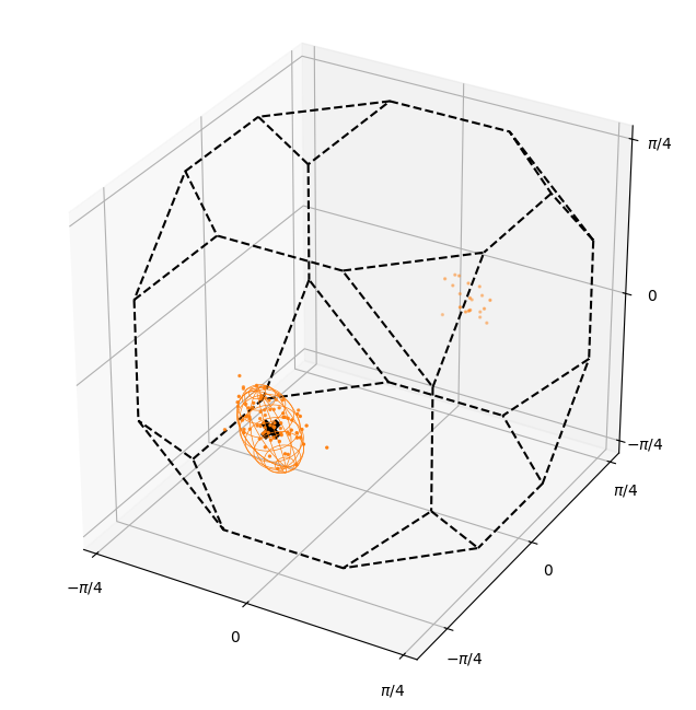
To test the method, we compare it to a method based on quaternion-statistics adapted from Pantleon 2005 by drawing from an oblate Bingham distribution and fitting both the mean orientation and the preferred misorientation axis and see how large of an error the two methods make on average.

from tqdm import tqdm

def cluster_of_rotations(N, g_mean, sigma_deg, prolate_direction=np.array([0,0,1])):
    sigma_rad = sigma_deg*np.pi/180
    random_quat = np.random.multivariate_normal(np.array([0, 0, 0, 1]),
                                                 np.diag(((sigma_rad/3)**2/np.pi, (sigma_rad/3)**2/np.pi, sigma_rad**2/np.pi, 0)),
                                                 size=(N))

    random_quat = random_quat / np.linalg.norm(random_quat, axis = 1)[:, np.newaxis]
    random_ori = R.from_quat(random_quat)
    R1 = R.from_euler('yz', [np.arccos(prolate_direction[2]), np.arctan2(prolate_direction[1], prolate_direction[0])])
    ori =  R1 * random_ori * R1.inv() *g_mean
    return ori

def do_one_sample(sigma, N):

    # Draw sample
    g2 = grids.random_quarternions(2)
    mean_ori = g2[0]
    anis_dir = g2[1].apply( np.array([0,0,1]))
    g_data = cluster_of_rotations(N, mean_ori, sigma, anis_dir)

    # Harmonics based analysis
    g_mean_formharm, c_fromharm = compute_cluster_statistics(g_data, 'cubic')
    eigval, eigvec =  np.linalg.eig(c_fromharm)
    main_eig_indx = np.argmax(np.abs(eigval))
    anis_dir_fromharm = eigvec[:, main_eig_indx]
    error_g_harm = np.min([(g_mean_formharm * s * g_data.inv()).magnitude() for s in point_groups.cubic])
    error_dir_harm = np.arccos(np.abs(np.dot(anis_dir_fromharm, anis_dir)))

    # Quaternion based analysis
    g_data_niceframe = mean_ori.inv() * g_data  # Cheat and use the ground-truth for resolving the symmetry identification
    quats = g_data_niceframe.as_quat()
    mean_quat = np.mean(quats, axis = 0)
    mean_quat = mean_quat / np.linalg.norm(mean_quat)
    g_quat = R.from_quat(mean_quat)
    R_quat = g_quat.as_matrix()
    error_g_quat = g_quat.magnitude()
    C_quat = quats.T @ quats / N
    eigval, eigvec =  np.linalg.eig(C_quat)
    anis_dir_fromquat = mean_ori.apply(eigvec[:-1,1])
    error_dir_quat = np.arccos(np.abs(np.dot(anis_dir_fromquat, anis_dir)))

    return error_g_harm, error_dir_harm, error_g_quat, error_dir_quat

# Run the experiment
N_samples = 200 # number of samples per experiment
N_experiments = 100
spread = 5 # Orientation spread in degrees

ghe_list = []; dhe_list = []; gqe_list = []; dqe_list = []
for ii in tqdm(range(N_experiments)):
    ghe, dhe, gqe, dqe = do_one_sample(spread, N_samples)
    ghe_list.append(ghe)
    dhe_list.append(dhe)
    gqe_list.append(gqe)
    dqe_list.append(dqe)

  0%|          | 0/100 [00:00<?, ?it/s]/home/madsac/miniconda3/envs/odftt/lib/python3.13/site-packages/odftomo/analysis/harmonics_fitting.py:70: UserWarning: Gimbal lock detected. Setting third angle to zero since it is not possible to uniquely determine all angles.
  gradient, resnorm = self.gradient(g_x, h_x)
100%|██████████| 100/100 [00:04<00:00, 20.73it/s]

# PLot the results
ax = plt.subplot(2,2,1)
ax.hist(np.array(ghe_list)*180/np.pi, range = (0, 2), color = [0.5, 0.5, 0.5])

ylims = [0, 45]
tt = [0, 0.5, 1, 1.5, 2]
ax.set_xticks(tt)
ax.set_xticklabels([f'{t}°' for t in tt])
ax.set_ylim(ylims)
plt.title('Centroid ori. error', fontsize=15)
plt.ylabel('Harmonics\nembedding', fontsize=15)
plt.plot([np.mean(ghe_list)*180/np.pi]*2, ylims, 'k--')

ax = plt.subplot(2,2,2)
ax.hist(np.array(dhe_list)*180/np.pi, range = (0, 10), color = [0.5, 0.5, 0.5])
tt = [0, 2, 4, 6, 8, 10]
ax.set_xticks(tt)
ax.set_xticklabels([f'{t}°' for t in tt])
ax.set_ylim(ylims)
plt.plot([np.mean(dhe_list)*180/np.pi]*2, ylims, 'k--')
plt.title('Pref. misori. axis error', fontsize=15)

ax = plt.subplot(2,2,3)
ax.hist(np.array(gqe_list)*180/np.pi, range = (0, 2), color = [0.5, 0.5, 0.5])
tt = [0, 0.5, 1, 1.5, 2]
ax.set_xticks(tt)
ax.set_xticklabels([f'{t}°' for t in tt])
ax.set_ylim(ylims)
plt.plot([np.mean(gqe_list)*180/np.pi]*2, ylims, 'k--')
plt.ylabel('Quaternions', fontsize=15)

ax = plt.subplot(2,2,4)
ax.hist(np.array(dqe_list)*180/np.pi, range = (0, 10), color = [0.5, 0.5, 0.5])
plt.plot([np.mean(dqe_list)*180/np.pi]*2, ylims, 'k--')
tt = [0, 2, 4, 6, 8, 10]
ax.set_xticks(tt)
ax.set_xticklabels([f'{t}°' for t in tt])
ax.set_ylim(ylims)
plt.show()

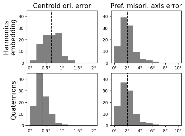
We see that the harmonics embedding approach does worse than the quaternions but not much worse. My theory is that the gradient-descent algoirithm does not work very well.

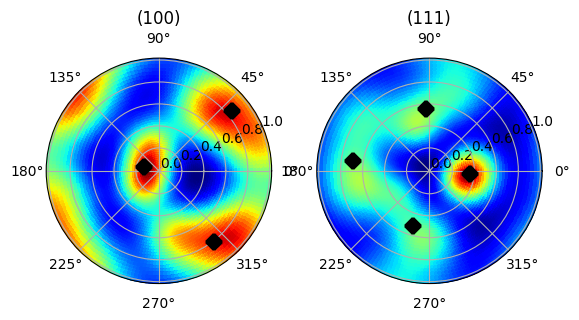
Another convenient use of the harmonics based function is that we can find the mean orientation of GSH reconstruction without needing to evaluate on a grid basis. I’m at the moment unaware of any other solution to that problem.

We simply replace the mean embedded harmonics with the embedding harmonics convolved with the ODF, which is a simple matrix product in GSH basis. We then proceed to solve the same low-dimensional optimization problem as before.

This is implemented in odftomo.analysis.harmonics_fittingMeanOrientationFinderGSH and we demonstrate with simulated data:

# Make simulated GSH data
from odftomo.spharm.RBF_mapper import kernel_function_to_kernel_coeff, RBF_to_GSH
from odftomo.analysis.harmonics_fitting import MeanOrientationFinderGSH
from odftomo.spharm.symmetrized_harmonics_coefficients import make_symmetrized_harmonics
from types import SimpleNamespace

# Draw some random orientation
random_orientations = grids.random_quarternions(2)
random_direction = random_orientations[1].apply([1, 0, 0])
g_cluster = draw_rotations(10, random_orientations[0], 20 , random_direction)

# Transform into full GSH-basis
def kernel_function(angles):
    return np.exp(-angles**2/2/0.3**2)

ell_max = 32

# Make a mock ODF object
odf_mock = SimpleNamespace(
    grid=g_cluster,
    pf_kernel=kernel_function,
    point_group=point_groups.cubic,
)

GSH_data = RBF_to_GSH(np.ones(len(g_cluster)), odf_mock, ell_max)

# Reduce to symmetrized-harmonics basis (the output format of TT reconstructions)
cube_harmonics = make_symmetrized_harmonics(ell_max, 'cubic')
odf_GSH = odfs.Harmonics(ell_max, cube_harmonics, point_groups.cubic)

sym_coeffs = np.zeros(odf_GSH.n_modes)
for mode_index in range(odf_GSH.n_modes):
    ell = odf_GSH.mode_coefficients[mode_index].ell
    sym_coeffs[mode_index] = np.sum(odf_GSH.mode_coefficients[mode_index].coefficients * GSH_data[ell])

/tmp/ipykernel_47031/113671976.py:25: UserWarning: Gimbal lock detected. Setting third angle to zero since it is not possible to uniquely determine all angles.
  GSH_data = RBF_to_GSH(np.ones(len(g_cluster)), odf_mock, ell_max)

# Do the orientation fitting
h = embedding_harmonics['cubic'][0].coefficients
ell = embedding_harmonics['cubic'][0].ell
ori_finder = MeanOrientationFinderGSH(odf_GSH, h, ell)
main_ori= ori_finder.find(sym_coeffs)

/home/madsac/miniconda3/envs/odftt/lib/python3.13/site-packages/odftomo/analysis/harmonics_fitting.py:70: UserWarning: Gimbal lock detected. Setting third angle to zero since it is not possible to uniquely determine all angles.
  gradient, resnorm = self.gradient(g_x, h_x)

# Plot the results
ax2 = plt.subplot(1,2,1,polar=True)
polefigure, map_theta, map_phi = odf_GSH.make_polefigure_map(sym_coeffs, np.array([1,0,0])/np.sqrt(1))
img = ax2.pcolormesh(map_phi, np.tan(map_theta/2), polefigure, edgecolors = 'face', rasterized = True, cmap = 'jet')
plt.title('(100)')
for pole in [np.array([1, 0, 0]),
             np.array([0, 1, 0]),
             np.array([0, 0, 1]),]:
    v = main_ori.apply(pole)
    if v[2] <= 0.0:
        v = -v
    plt.plot(np.arctan2(v[1], v[0]), np.tan(np.arccos(v[2])/2), 'kx', markeredgewidth = 10)

ax2 = plt.subplot(1,2,2,polar=True)
polefigure, map_theta, map_phi = odf_GSH.make_polefigure_map(sym_coeffs, np.array([1,1,1])/np.sqrt(3))
img = ax2.pcolormesh(map_phi, np.tan(map_theta/2), polefigure, edgecolors = 'face', rasterized = True, cmap = 'jet')
plt.title('(111)')
for pole in [np.array([1, 1, 1])/np.sqrt(3),
             np.array([-1, 1, 1])/np.sqrt(3),
             np.array([1, -1, 1])/np.sqrt(3),
             np.array([1, 1, -1])/np.sqrt(3)]:
    v = main_ori.apply(pole)
    if v[2] <= 0.0:
        v = -v
    plt.plot(np.arctan2(v[1], v[0]), np.tan(np.arccos(v[2])/2), 'kx', markeredgewidth = 10)
plt.show()