Grain segmentation workflow

This notebook demonstrates how the simple grain-segmentation workflow is called using the rolled-steel dataset that was created by the end of the Data corrections notebook.

Basic reconstruction

Before we can do the grain-segmentation, we have to make a reconstruction. This is done with the standard RBF workflow.

import numpy as np
from tqdm import tqdm
from odftomo.texture import grids, point_groups, odfs
from odftomo.tomography_models import FromArrayModel
from odftomo.crystallography import cubic
from odftomo.optimization import FISTA
from scipy.spatial.transform import Rotation as R

import matplotlib.pyplot as plt
from odftomo import plot_tools
from mumott import Geometry
import h5py
from odftomo.analysis.segmentation import find_texture_components, grain_segmentation

import logging
logger = logging.getLogger()
logger.setLevel(logging.ERROR)

INFO:Setting the number of threads to 4. If your physical cores are fewer than this number, you may want to use numba.set_num_threads(n), and os.environ["OPENBLAS_NUM_THREADS"] = f"{n}" to set the number of threads to the number of physical cores n.
INFO:Setting numba log level to WARNING.

Load the data that was prepared in a different notebook.

# Save data
geom = Geometry()
geom.read('data/iron_slice.mumottgeometry')

with h5py.File(f'data/fe3si_65_cw_layer_22_alpha_corrected.h5', 'r') as file:

    rot_angles = np.array(file['rotangle_degrees'])
    azi_angles = np.array(file['aziangle_degrees'])
    data_array = np.array(file['data_array'])
    twotheta_list = np.array(file['twotheta_list'])
    hkl_list = np.array(file['hkl_list'])

hkl_list = [tuple(hkl) for hkl in hkl_list]

# Compute sample-coordinates-q-vector probed for each data point.
coordinates = []
for twotheta in twotheta_list:
    geom.two_theta = twotheta * np.pi / 180
    coordinates.append(geom.probed_coordinates.vector[:,:,1,:])
coordinates = np.stack(coordinates, axis = -1)
coordinates = coordinates.transpose((0,1,3,2))[:,np.newaxis,np.newaxis,:,:,:]

grid_resolution_parameter = 25
grid = grids.hopf_grid(grid_resolution_parameter, point_groups.cubic)
odf = odfs.GaussianRBF(grid, point_groups.cubic)
print(f'The grid contains {odf.n_modes} orientations.')

A, B = cubic()
h_vectors = [B @ hkl for hkl in hkl_list]
basis_function_arrays = odf.compute_polefigure_matrices_parallel(coordinates, h_vectors, num_processes=4)
model = FromArrayModel(basis_function_arrays, geom)

The grid contains 2568 orientations.
Starting parallel computation of polefiugres.

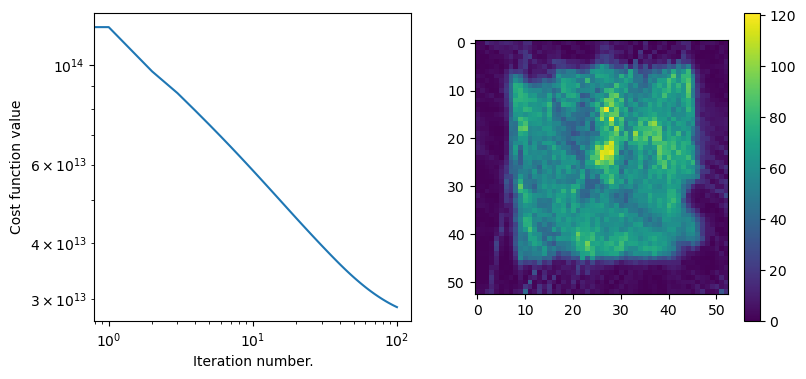
optimizer = FISTA(model, data_array, maxiter = 100)
coefficients, convergence_curve = optimizer.optimize()

fig = plt.figure(figsize = (9,4))
plt.subplot(1,2,1)
plt.loglog(convergence_curve)
plt.xlabel('Iteration number.')
plt.ylabel('Cost function value')

plt.subplot(1,2,2)
plt.imshow(np.sum(coefficients, axis = -1))
plt.colorbar()
plt.show()

Estimating largest safe step size

Matrix norm estimate = 1.01E+10:  30%|███       | 3/10 [00:03<00:08,  1.23s/it]
Loss = 2.88E+13: 100%|██████████| 100/100 [01:37<00:00,  1.02it/s]

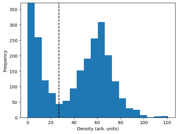
mask_threshold = 27

dens = np.sum(coefficients, axis = -1)
mask = dens > mask_threshold
freq = plt.hist(dens.flatten(), bins = 20)[0]
plt.ylim(0, np.max(freq[5:])*1.2)
plt.plot([mask_threshold]*2, [0, np.max(freq[5:])*1.2], 'k--')
plt.xlabel('Density (arb. units)')
plt.ylabel('Frequency')
plt.show()

Find voxel-by-voxel texture components

The clustering algorithm has three tuneable parameters:

1. A theshold weight. I usually use some large fraction of the weight used to mask sample from air.

2. A radius. The typical radius of a texture component. Any grid mode within this distance is considered part of the same texture component. It should be significantly larger than the grid resolution.

3. Max number of texture components per voxel. Usually not important if the threshold is set high enough.

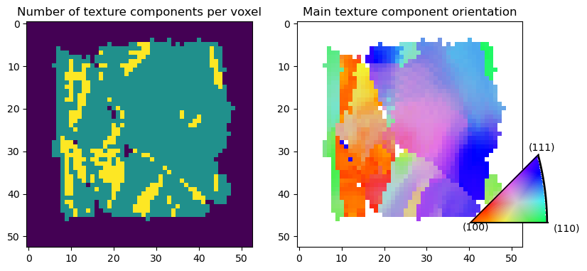
# Find texture components in each voxel
texture_component_tomogram = find_texture_components(
    coefficients,
    odf,
    density_threshold = 0.5*mask_threshold,
    texture_component_radius = 10.0,
)

/das/home/carlse_m/grids_in_so3/odftt/analysis/grid_tools.py:113: RuntimeWarning: invalid value encountered in arccos
  dist_this = np.arccos(2*np.abs(np.einsum('ik,k->i',
100%|██████████| 2809/2809 [00:54<00:00, 51.53it/s]

# For each pixel, store the main orientation
volume_shape = coefficients.shape[:-1]
rotvec_tomogram = np.zeros((*volume_shape, 3))
IFP_direction = np.array([1, 0, 0])
for ii in tqdm(range(volume_shape[0])):
    for jj in range(volume_shape[1]):
        for kk in range(volume_shape[2]):
            if texture_component_tomogram[ii,jj,kk,0] != 0:
                rotvec_tomogram[ii, jj, kk, :] = texture_component_tomogram[ii,jj,kk,0].COM_ori.as_rotvec()

fig = plt.figure(figsize = (9,5))

plt.subplot(1,2,1)
plt.imshow(np.sum(texture_component_tomogram != 0, axis = -1)[:,:,0])
plt.title('Number of texture components per voxel')

plt.subplot(1,2,2)
rgb = plot_tools.IPF_color(rotvec_tomogram, IFP_direction, 'cubic')
mask = np.any(texture_component_tomogram != 0, axis = -1)
rgb[~mask, :] = 1
plt.imshow(rgb[:,:,0])
plt.title('Main texture component orientation')
ax = fig.add_subplot([0.75, 0.20, 0.30, 0.30], polar = True)
plot_tools.make_color_legend(ax, 'cubic')
fig.show()

100%|██████████| 53/53 [00:00<00:00, 5186.73it/s]

Collect texture component into grains

The grain-segmentation function takes the output of the texture-component clustering output. There is one further tunable parameter, which is the a distance threshold when comparing neighboring voxels

sorted_grains_list = grain_segmentation(
    texture_component_tomogram,
    distance_threshold=7.0,
    point_group=odf.point_group,
)

/das/home/carlse_m/grids_in_so3/odftt/analysis/grid_tools.py:113: RuntimeWarning: invalid value encountered in arccos
  dist_this = np.arccos(2*np.abs(np.einsum('ik,k->i',

grain_number = 0
fig = plt.figure(figsize = (9, 12))

grain_index = np.zeros(geom.volume_shape)
main_grain_dens = np.zeros(geom.volume_shape)

for index, grain in enumerate(sorted_grains_list):
    where = grain.density > main_grain_dens
    grain_index[where] = index
    main_grain_dens[where] = grain.density[where]
grain_index[main_grain_dens==0] = np.nan

ax = plt.subplot(4,3,1)
plt.imshow(grain_index[:,:,0]%10, cmap = 'Set1', interpolation = 'nearest')
plt.title('Grain index')
ax.grid()


for grain in sorted_grains_list[:11]:
    ax = plt.subplot(4,3,grain_number+2)
    ax.imshow(np.sum(grain.density, axis=2))
    ax.set_title(f'Grain #{grain_number}')
    ax.grid()
    bbox = grain.bbox_voxel
    ax.plot([bbox[2], bbox[2], bbox[3], bbox[3], bbox[2]], [bbox[0], bbox[1], bbox[1], bbox[0], bbox[0]], '--w')
    grain_number+=1
plt.show()

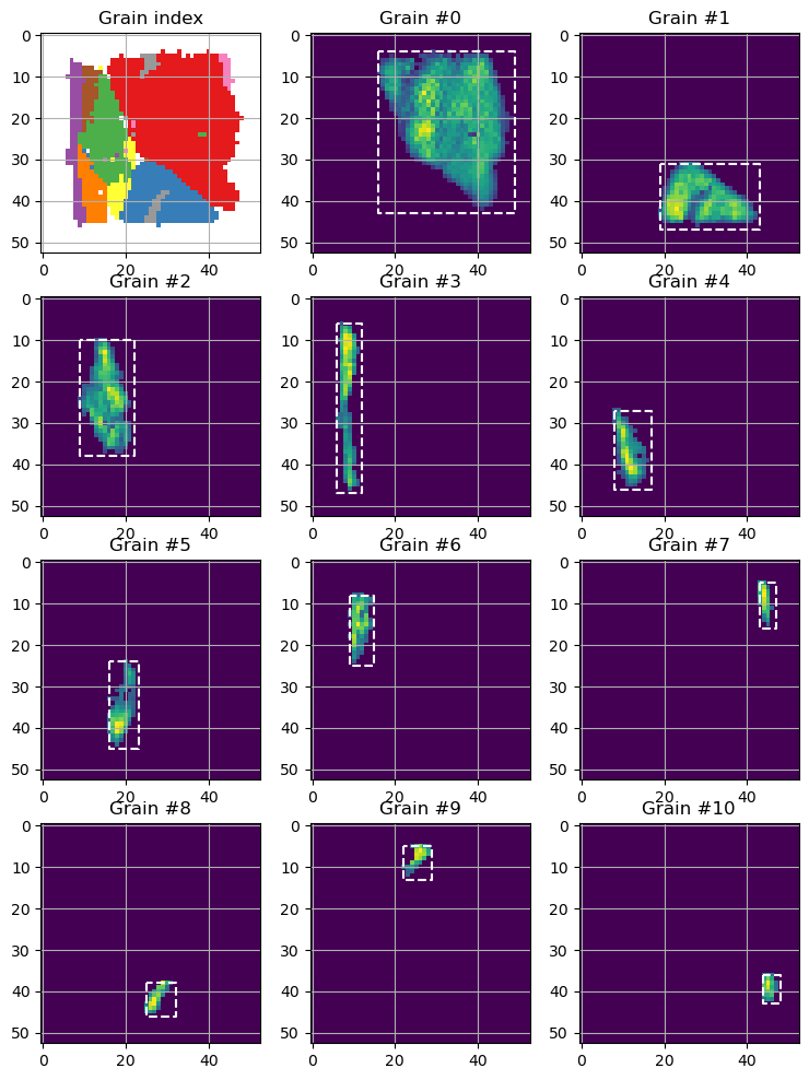
The information contained in each grain is now:

1. Orientation field

2. Density field

3. Orientation space bounding box

4. Real space bounding box

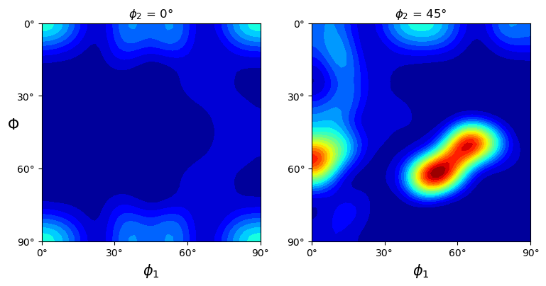
Euler angle sections in Bunge convention

# Change coordinate system
from odftomo.spharm.RBF_mapper import RBF_mapper

Psi = np.array([0, -np.pi/4])
Theta = -np.linspace(0, np.pi/2, 46, endpoint=True)
Phi = np.linspace(0, np.pi/2, 46, endpoint=True)

# Transform from laboratory coordinate system to conventional rolling-texture system
ND = np.array([0, 1, 0]); RD = np.array([0, 0, 1]); TD = np.array([1, 0, 0])
g_transform = R.from_matrix(np.stack([RD, TD, -ND])) # Transform from lab coordinates to conventional rolling-texture coords.

mean_texture = np.mean(coefficients, axis=(0,1,2))
ODF_map, (Psi_map, Theta_map, Phi_map) = RBF_mapper(mean_texture,
                                                    odf,
                                                    euler_angles_tuple = (Psi, Theta, Phi),
                                                    strategy='spharm',
                                                    specimen_symmetry = [p*g_transform.inv() for p in point_groups.orthorhombic])

/das/home/carlse_m/grids_in_so3/odftt/spharm/RBF_mapper.py:87: UserWarning: Gimbal lock detected. Setting third angle to zero since it is not possible to uniquely determine all angles.
  transform = RBF_to_GSH(RBF_coeffs, odf_RBF, ell_max)
100%|██████████| 33/33 [00:03<00:00, 10.82it/s]

# Make nice plot (Bunge angle convention I think. Very stange!)
plt.figure(figsize = (9, 4))

for ii in range(2):
    plt.subplot(1,2,ii+1)
    plt.contourf(np.clip(ODF_map[ii,:,:], 0, np.inf), extent = (90, 0, 0, 90),
                 levels=np.linspace(0, np.max(ODF_map), 21), cmap='jet')
    plt.title(rf'$\phi_2$ = {np.abs(Psi[ii])*180/np.pi:.0f}°')
    ticks = [0, 30, 60, 90]; labels = ['0°', '30°', '60°', '90°']
    plt.xticks(ticks, labels=labels)
    plt.yticks(ticks, labels=labels)
    plt.ylim(90, 0)
    plt.xlim(0, 90)
    plt.axis('scaled')
    if ii == 0:
        plt.ylabel(r'$\Phi$', rotation=0, fontsize = 15)
    plt.xlabel(r'$\phi_1$', fontsize = 15)

plt.show()