Computing the main orientation field

This notebook demontrates how to extract the orientation-field from reconstructions in cases where there is a single dominant orientation in each voxel of the reconstructions.

To demonstrate this, we use data from a Roman snail shell sample. The experiment is descibed in https://arxiv.org/abs/2407.11022. The data is availible at https://zenodo.org/records/14800063.

To download:

wget https://zenodo.org/records/14800063/files/aragonite_012.h5 https://zenodo.org/records/14800063/files/aragonite_021.h5 https://zenodo.org/records/14800063/files/aragonite_041.h5 https://zenodo.org/records/14800063/files/aragonite_111.h5 https://zenodo.org/records/14800063/files/aragonite_132.h5 https://zenodo.org/records/14800063/files/aragonite_211.h5 https://zenodo.org/records/14800063/files/aragonite_221.h5 https://zenodo.org/records/14800063/files/aragonite_012.h5

Imports

import matplotlib as mpl
import matplotlib.pyplot as plt
import numpy as np
from scipy.spatial.transform import Rotation as R
from tqdm import tqdm
from odftomo.io import load_series, slice_geometry
from odftomo.texture import grids, point_groups, odfs
from odftomo.tomography_models import FromArrayModel
from odftomo.crystallography import orthorhombic
from odftomo.optimization import FISTA
import odftomo.plot_tools
from odftomo.analysis.grid_tools import distance_matrix, mean_orientations_inside_radius
from odftomo.analysis.segmentation import blob_finder

import logging
logger = logging.getLogger()
logger.setLevel(logging.ERROR)

INFO:Setting the number of threads to 4. If your physical cores are fewer than this number, you may want to use numba.set_num_threads(n), and os.environ["OPENBLAS_NUM_THREADS"] = f"{n}" to set the number of threads to the number of physical cores n.
INFO:Setting numba log level to WARNING.

Run reconstruction

In order to demonstrate the analysis, we first need a reconstruction. For an explaination of the reconstruction workflow, see one of the other notebooks.

# Load data files
hkl_list = [(1, 1, 1), (0, 2, 1), (0, 1, 2), (2, 1, 1), (2, 2, 1), (0, 4, 1), (1, 3, 2),]
files = [f'aragonite_{h[0]}{h[1]}{h[2]}.h5' for h in hkl_list]
data_array, weigth_array, coordinates, full_geom = load_series(files)

data_array[np.isnan(data_array) ] = 0
data_array[np.isinf(data_array) ] = 0

/das/home/carlse_m/mumott_dev_version/mumott/mumott/data_handling/data_container.py:227: DeprecationWarning: Entry name rotations is deprecated. Use inner_angle instead.
  _deprecated_key_warning('rotations')
/das/home/carlse_m/mumott_dev_version/mumott/mumott/data_handling/data_container.py:236: DeprecationWarning: Entry name tilts is deprecated. Use outer_angle instead.
  _deprecated_key_warning('tilts')
/das/home/carlse_m/mumott_dev_version/mumott/mumott/data_handling/data_container.py:268: DeprecationWarning: Entry name offset_j is deprecated. Use j_offset instead.
  _deprecated_key_warning('offset_j')
/das/home/carlse_m/mumott_dev_version/mumott/mumott/data_handling/data_container.py:278: DeprecationWarning: Entry name offset_k is deprecated. Use k_offset instead.
  _deprecated_key_warning('offset_k')
/das/home/carlse_m/grids_in_so3/odftt/io/mumott_fileformat_loader.py:26: RuntimeWarning: divide by zero encountered in divide
  data_arrays.append(np.array(data_container.data / data_container.diode[:, :, :, np.newaxis]))
/das/home/carlse_m/grids_in_so3/odftt/io/mumott_fileformat_loader.py:26: RuntimeWarning: invalid value encountered in divide
  data_arrays.append(np.array(data_container.data / data_container.diode[:, :, :, np.newaxis]))

Reduce the full 3D dataset to a single 2D slice. This is done to make the reconstruction faster for this demonstration to run easily on slow hardware.

# Reduce the dataset to only the zero tilt part
data_array = data_array[:50, ...]
weigth_array = weigth_array[:50, ...]
coordinates = coordinates[:50, ...]
geom = slice_geometry(full_geom, slice(50))

# crop out a singe slice of the data
data_slice = data_array[:,:,24:25,:,:]
weigth_slice = weigth_array[:,:,24:25,:,:]

# Make a geometry object for the single-slice reconstructions
from mumott.core.geometry import Geometry, GeometryTuple
geom_slice = Geometry()

for gt in geom:
    gt_new = GeometryTuple(rotation = gt.rotation, k_offset = 0.0, j_offset = 0)
    geom_slice.append(gt_new)

geom_slice.volume_shape = np.array([60, 1, 60])
geom_slice.projection_shape = np.array([54, 1])
geom_slice.p_direction_0 = geom.p_direction_0
geom_slice.j_direction_0 = geom.j_direction_0
geom_slice.k_direction_0 = geom.k_direction_0
geom_slice.detector_direction_origin = geom.detector_direction_origin
geom_slice.detector_direction_positive_90 = geom.detector_direction_positive_90
geom_slice.detector_angles = geom.detector_angles
geom_slice.full_circle_covered = geom.full_circle_covered

# Normalize data by aproximated formfactor
scale = np.mean(data_array, axis = (0, 1, 2, 3))
data_slice = data_slice / scale[np.newaxis, np.newaxis, np.newaxis, np.newaxis, :]

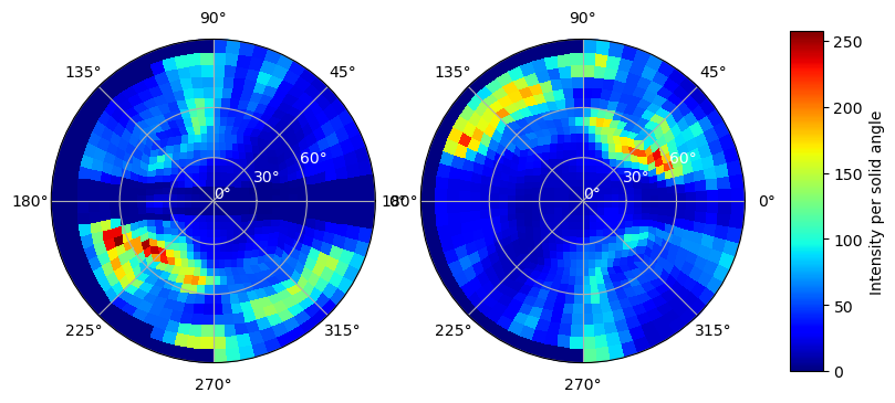
Looking at the experimental data, e.g. an experimental polefigure averaging over a 2D slice, the sample appears to have a continuous texture and not single orientations.

# Look at the raw data
hkl_index = 1
fig, axs = odftomo.plot_tools.plot_experimental_polefigure(np.sum(data_slice[...,hkl_index], axis =(1,2)),
                                                         coordinates[...,hkl_index,:],
                                                         resolution_in_degrees=5)

fig.show()

/das/home/carlse_m/grids_in_so3/odftt/plot_tools/data_plots.py:24: RuntimeWarning: invalid value encountered in divide
  histogram = intens_histograms[ii][0] / norm_histograms[ii][0]

Set up the objects needed for the full reconstruction model

# Define a model of the ODF
grid_resolution_parameter = 15
kernel_sigma = 0.1
grid = grids.hopf_grid(grid_resolution_parameter, point_groups.orthorhombic)
odf = odfs.GaussianRBF(grid, point_groups.orthorhombic, kernel_sigma)

# Find probed lattice vectors
A, B = orthorhombic(a = 4.960, b = 7.964, c = 5.738)
h_vectors = [B @ hkl for hkl in hkl_list]

# Set up full forward model
basis_function_arrys = odf.compute_polefigure_matrices_parallel(coordinates, h_vectors, num_processes=4)
model = FromArrayModel(basis_function_arrys, geom_slice)

Starting parallel computation of polefiugres.

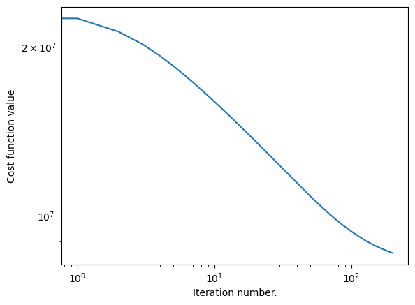
Run the actual reconstruction

# Run actual reconstruction
optimizer = FISTA(model, data_slice, weights=weigth_slice, maxiter=200, regularization_weigth=1e4)
coefficients, convergence_curve = optimizer.optimize()

plt.loglog(convergence_curve)
plt.xlabel('Iteration number.')
plt.ylabel('Cost function value')
plt.show()

Estimating largest safe step size

Matrix norm estimate = 1.65E+08:  20%|██        | 2/10 [00:03<00:13,  1.67s/it]
Loss = 8.59E+06: 100%|██████████| 200/200 [04:05<00:00,  1.23s/it]

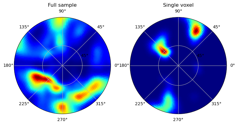
We check that the reconstruction reconstructs the mean texture of the whole slice well. The computes polefigures are guarantees symmetric, so we only plot the top half sphere.

# PLot reconstructed pole figure
mean_texture = np.mean(coefficients, axis = (0, 1, 2))
h_vector =  B @ hkl_list[hkl_index]
h_vector = h_vector / np.linalg.norm(h_vector)
mean_pf = polefigure, theta_grid, phi_grid = odf.make_polefigure_map(mean_texture, h_vector)

fig = plt.figure(figsize = (9, 4.5))
ax = plt.subplot(1, 2, 1, polar=True)
img = ax.pcolormesh(phi_grid, np.tan(theta_grid/2), polefigure, rasterized=True, cmap = 'jet')
ax.set_yticks([np.tan(ii*np.pi/8) for ii in range(1, 2)])
ax.set_yticklabels(['45°'])
ax.yaxis.label.set_color('w')
plt.title(f'{hkl_list[hkl_index][0]}{hkl_list[hkl_index][1]}{hkl_list[hkl_index][2]} Pole figure\nPositive z')
ax.set_title('Full sample')

voxel_texture = coefficients[34, 0, 28, :]
voxel_pf = polefigure, theta_grid, phi_grid = odf.make_polefigure_map(voxel_texture, h_vector)

ax = plt.subplot(1, 2, 2, polar=True)
img = ax.pcolormesh(phi_grid, np.tan(theta_grid/2), polefigure, rasterized=True, cmap = 'jet')
ax.set_yticks([np.tan(ii*np.pi/8) for ii in range(1,2)])
ax.set_yticklabels(['45°'])
ax.yaxis.label.set_color('w')
plt.title(f'{hkl_list[hkl_index][0]}{hkl_list[hkl_index][1]}{hkl_list[hkl_index][2]} Pole figure\nPositive z')
ax.set_title('Single voxel')
plt.savefig('../img/snail_pole_figures.png')
plt.show()

Analyze and visualize reconstruction

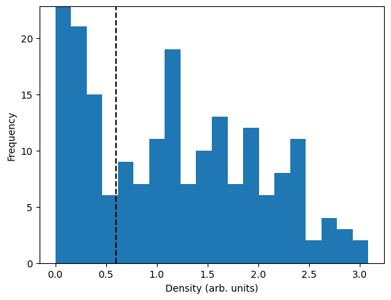
First we pick a threshold value to mask the regions containing sample.

# Pick a threshold value to determine what pixels to plot.
mask_threshold = 0.6

dens = np.sum(coefficients, axis=-1)
mask = dens > mask_threshold
freq = plt.hist(dens.flatten(), bins = 20)[0]
plt.ylim(0, np.max(freq[5:])*1.2)
plt.plot([mask_threshold]*2, [0, np.max(freq[5:])*1.2], 'k--')
plt.xlabel('Density (arb. units)')
plt.ylabel('Frequency')
plt.show()

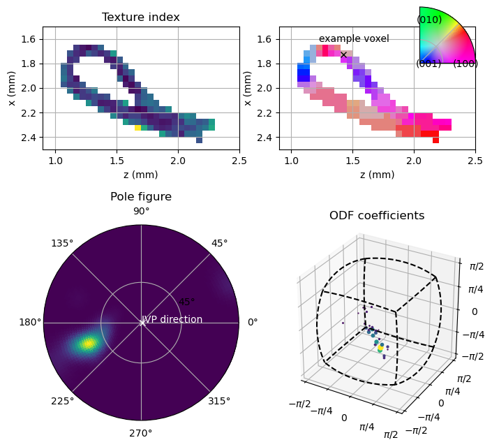
Here we plot a number of tomograms of computed quantities.

The main quantity of interest is the max_orientation which is the orientation for each voxel that corresponds to the largest coefficient in the reconstruction.

# Some options for defining the plot
IVP_map_direction = np.array([0, 0, 1])
pole_figure_hkl = np.array([0, 0, 1])
example_voxel = (34, 0, 28)
stepsize = 0.05
pcolor_opts = {'edgecolors':'face', 'vmin':0, 'rasterized':True}
imshow_opts = {'extent':(0,coefficients.shape[2]*stepsize,coefficients.shape[0]*stepsize,0)}

def tomogram_set_axes(ax):
    ax.set_xlabel('z (mm)')
    ax.set_ylabel('x (mm)')
    ax.set_xlim(0.9, 2.5);
    ax.set_ylim(2.5, 1.5)
    ax.grid()

main_orientation_tomogram = odf.main_orientation(coefficients)
ipf_rgb_tomogram = odftomo.plot_tools.IPF_color(main_orientation_tomogram, IVP_map_direction, 'orthorhombic')
ipf_rgb_tomogram[~mask, :] = 1

# Compute approximate texture index
J = np.sqrt(np.var(coefficients, axis = -1)) / np.mean(coefficients, axis = -1)
J[~mask] = np.nan

# Compute a pole-figure of a single voxel
voxel_coeffs = coefficients[example_voxel[0], example_voxel[1], example_voxel[2],:]
polefigure, theta_grid, phi_grid = odf.make_polefigure_map(voxel_coeffs, B @ pole_figure_hkl)

/tmp/ipykernel_272035/1637345821.py:21: RuntimeWarning: invalid value encountered in divide
  J = np.sqrt(np.var(coefficients, axis = -1)) / np.mean(coefficients, axis = -1)

# Build the plot
fig = plt.figure(figsize = (8, 8))

# PLot IVP-map
ax = plt.subplot(2,2,2)
ax.imshow(ipf_rgb_tomogram[:, 0, :], **imshow_opts)
ax.plot((example_voxel[2]+0.5)*stepsize, (example_voxel[0]+0.5)*stepsize, 'kx')
ax.text((example_voxel[2]+0.5)*stepsize - 0.2, (example_voxel[0]+0.5)*stepsize - 0.1, 'example voxel', color = 'k')
tomogram_set_axes(ax)
ax = fig.add_subplot([0.8, 0.75, 0.10, 0.10], polar = True)
odftomo.plot_tools.make_color_legend(ax, 'orthorhombic')

# Plot texture index
ax = plt.subplot(2,2,1)
img = ax.imshow(J[:, 0, :], **imshow_opts)
tomogram_set_axes(ax)
ax.set_title('Texture index')

# PLot pole figure
ax = plt.subplot(2,2,3, polar=True)
img = ax.pcolormesh(phi_grid, np.tan(theta_grid/2), polefigure, **pcolor_opts)
ax.set_yticks([np.tan(ii*np.pi/8) for ii in range(1,2)])
ax.set_yticklabels(['45°'])
ax.yaxis.label.set_color('w')
ax.set_title('Pole figure')
if IVP_map_direction[2] < 0.0:
    IVP_map_direction = -IVP_map_direction
IVP_map_theta = np.arctan2(np.sqrt(IVP_map_direction[0]**2+IVP_map_direction[1]**2), IVP_map_direction[2])
IVP_map_phi = np.arctan2(IVP_map_direction[1], IVP_map_direction[0])
ax.plot(IVP_map_phi, np.tan(IVP_map_theta/2), 'wx')
ax.text(IVP_map_phi+0.3, np.tan(IVP_map_theta/2), 'IVP direction',color = 'w')

# PLot ODF modes in Rodriguez-vector representation
ax = plt.subplot(2,2,4, projection='3d')
voxel_coeffs = coefficients[example_voxel[0], example_voxel[1], example_voxel[2],:]
odftomo.plot_tools.plot_orientation_coeffs(voxel_coeffs, odf.grid, ax, point_group_string='orthorhombic')
ax.set_title('ODF coefficients')
fig.tight_layout()
fig.show()

/tmp/ipykernel_272035/106017968.py:38: UserWarning: This figure includes Axes that are not compatible with tight_layout, so results might be incorrect.
  fig.tight_layout()
/tmp/ipykernel_272035/106017968.py:38: UserWarning: Tight layout not applied. The left and right margins cannot be made large enough to accommodate all Axes decorations.
  fig.tight_layout()

While the max-orientation generally gives a decent estimate of the main orientation in each voxel that can be used for plotting, it always snaps to one of the grid orientations, and can therefore give a blocky-looking orientation field, where the underlying reconstruction varies slowly. We can improve the orientation by including the influence of other orientations in the neighborhood of the max mode. We do this by selecting all modes withing a certain radius of the main orientation and computing a weighted average of these orientations (in a tangent space centered on the max orientation, where the average can be defined)

In a first step towards this, we compute the distance_matrix which contains the distances between all pairs of orientations in the grid. For large grids, this is an expensive calculation but it can in principle be re-used if the same grid is used many times.

main_orientation_tomogram = odf.main_orientation(coefficients, method='COM', radius=20.0)
ipf_rgb_tomogram_mean = odftomo.plot_tools.IPF_color(main_orientation_tomogram, IVP_map_direction, 'orthorhombic')
ipf_rgb_tomogram_mean[~mask, :] = 1

4it [00:00, 157.80it/s]
605it [00:00, 1057.70it/s]

fig = plt.figure(figsize = (9, 3))
ax = plt.subplot(1,2,1)
plt.imshow(ipf_rgb_tomogram[:, 0, :],**imshow_opts)
plt.title('Max coeff orientation')
tomogram_set_axes(ax)
ax.plot((example_voxel[2]+0.5)*stepsize, (example_voxel[0]+0.5)*stepsize, 'kx')

ax = plt.subplot(1,2,2)
plt.imshow(ipf_rgb_tomogram_mean[:, 0, :],**imshow_opts)
tomogram_set_axes(ax)
ax.plot((example_voxel[2]+0.5)*stepsize, (example_voxel[0]+0.5)*stepsize, 'kx')
plt.title('Mean orientation')
ax = fig.add_subplot([0.75, 0.60, 0.25, 0.25], polar = True)
odftomo.plot_tools.make_color_legend(ax, 'orthorhombic')
plt.savefig('../img/snail_orientation_field.png')
plt.show()

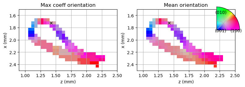
We see that the corrected mean-orientation is now more smooth on the IVP-map and in the Rodriguez-vector 3D scatter plot, we see that the computed mean oientation is somewhere between the orientations with the largest coefficients.

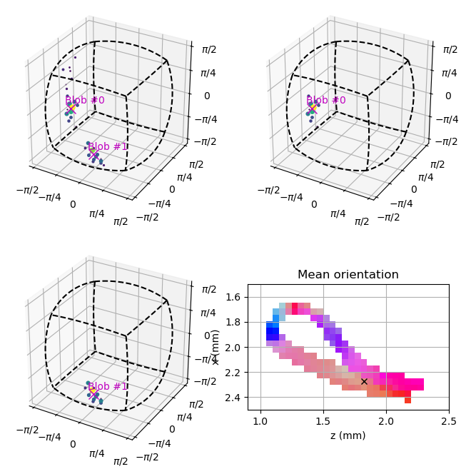
Mutiple blobs in a single voxel

Sometimes there are more than one texture-blob in a single voxel. Then we need to do some kind of clustering. The normal algorithms are a bit tricky to use, as we are not operating in a vector-space, but we have a simple implementation, which can be called voxel by voxel.

To demonstrate, let’s find a voxel with mutliple orientations:

example_voxel = (45, 0, 36)
voxel_coeffs = coefficients[example_voxel[0], example_voxel[1], example_voxel[2],:]
blob_list = blob_finder(voxel_coeffs, 0.5*mask_threshold, 30, grid, odf.point_group)

fig = plt.figure(figsize = (8, 8))
ax0 = plt.subplot(2,2,1,projection='3d')
odftomo.plot_tools.plot_orientation_coeffs(voxel_coeffs, odf.grid, ax0, point_group_string='orthorhombic')

for ii, blob in enumerate(blob_list):
    blob_ori = blob_list[ii].COM_ori.as_rotvec()
    ax0.plot(blob_ori[0], blob_ori[1], blob_ori[2], 'mx', markersize = 10)
    ax0.text(blob_ori[0], blob_ori[1]-0.3, blob_ori[2]+0.3, f'Blob #{ii}', color='m')

    ax_here = plt.subplot(2,2,2+ii,projection='3d')

    g = blob_list[ii].COM_ori
    dist = np.min(np.stack([(odf.grid*s*g.inv()).magnitude() for s in odf.point_group], axis = 1), axis=1)
    coeffs_in_texturecomponent = np.copy(voxel_coeffs)
    coeffs_in_texturecomponent[dist*180/np.pi > 30] = 0
    odftomo.plot_tools.plot_orientation_coeffs(coeffs_in_texturecomponent, odf.grid, ax_here, point_group_string='orthorhombic')
    ax_here.plot(blob_ori[0], blob_ori[1], blob_ori[2], 'mx', markersize = 10)
    ax_here.text(blob_ori[0], blob_ori[1]-0.3, blob_ori[2]+0.3, f'Blob #{ii}', color='m')

ax = plt.subplot(2,2,4)
plt.imshow(ipf_rgb_tomogram_mean[:, 0, :],**imshow_opts)
# plt.title('Mean orientation')
tomogram_set_axes(ax)
ax.plot((example_voxel[2]+0.5)*stepsize, (example_voxel[0]+0.5)*stepsize, 'kx')
plt.title('Mean orientation')
plt.show()

/das/home/carlse_m/grids_in_so3/odftt/analysis/grid_tools.py:112: RuntimeWarning: invalid value encountered in arccos
  dist_this = np.arccos(2*np.abs(np.einsum('ik,k->i',