Evaluate quality of reconstruction

This notebook demontrates how to plot the residuals of the reconstruction, which can be used to debug geometry problems and evaluate the quality of the reconstruction. But don’t over-rely on the residuals! Overfitting is a real problem and a better fit is not always a better reconstruction.

The data is from an in-house experiment at ID-11 at ESRF from August 2024.

Run reconstruction

In order to demonstrate the analysis, we first need a reconstruction. For an explaination of the reconstruction workflow, see one of the other notebooks.

import matplotlib.pyplot as plt
import matplotlib as mpl
import numpy as np
import odftomo.plot_tools
from tqdm import tqdm

from odftomo.io import load_series
from odftomo.texture import grids, point_groups, odfs
from odftomo.tomography_models import FromArrayModel
from odftomo.crystallography import hexagonal
from odftomo.optimization import FISTA
from odftomo.spharm.RBF_mapper import RBF_mapper

import logging
logger = logging.getLogger()
logger.setLevel(logging.ERROR)

INFO:Setting the number of threads to 4. If your physical cores are fewer than this number, you may want to use numba.set_num_threads(n), and os.environ["OPENBLAS_NUM_THREADS"] = f"{n}" to set the number of threads to the number of physical cores n.
INFO:Setting numba log level to WARNING.

# Load the data
hkl_list = [(1, 0, 0),
            (0, 0, 2),
            (1, 0, 1),
            (1, 0, 2),
            (1, 1, 0),
            (1, 0, 3),
            (1, 1, 2),
            (2, 0, 1),]
files = [f'data/Ti64/Ti64_smallslice_binned_{h[0]}{h[1]}{h[2]}.h5' for h in hkl_list]
data_array, weigth_array, coordinates, full_geom = load_series(files)

# Define reconstruction model
grid_resolution_parameter = 15 # This determines the numebr of grid points
grid = grids.hopf_grid(grid_resolution_parameter, point_groups.hexagonal)
odf_RBF = odfs.GaussianRBF(grid, point_groups.hexagonal)
print(f'The grid contains {odf_RBF.n_modes} orientations.')

# Define a lattice matrix with the correct orientation of the symmetry axes
A, B = hexagonal(a = 2.93, c = 4.66)
h_vectors = [B @ hkl for hkl in hkl_list] #  The hkl_list needs to be in 3-index format,
                                          #  not the special hexagonal 4 index system.
basis_function_arrys = odf_RBF.compute_polefigure_matrices_parallel(coordinates, h_vectors, num_processes=4)
model_RBF = FromArrayModel(basis_function_arrys, full_geom)

The grid contains 1159 orientations.
Starting parallel computation of polefiugres.

# Run actual optimization
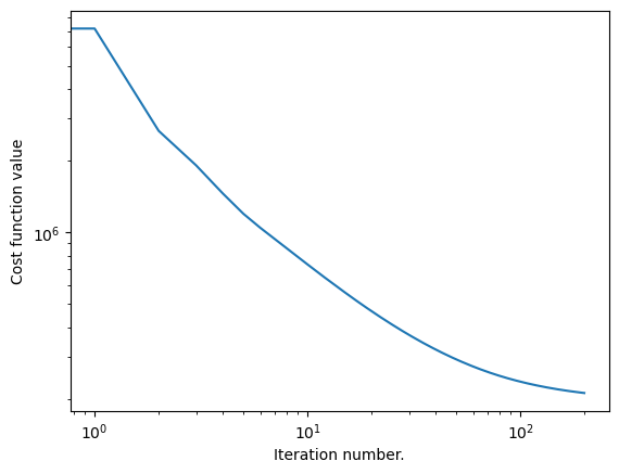
optimizer = FISTA(model_RBF, data_array, weights=weigth_array, maxiter=200)
coefficients, convergence_curve = optimizer.optimize()

plt.loglog(convergence_curve)
plt.xlabel('Iteration number.')
plt.ylabel('Cost function value')
plt.show()

Estimating largest safe step size

Matrix norm estimate = 1.91E+09:  20%|██        | 2/10 [00:01<00:04,  1.99it/s]
Loss = 2.12E+05: 100%|██████████| 200/200 [01:03<00:00,  3.13it/s]

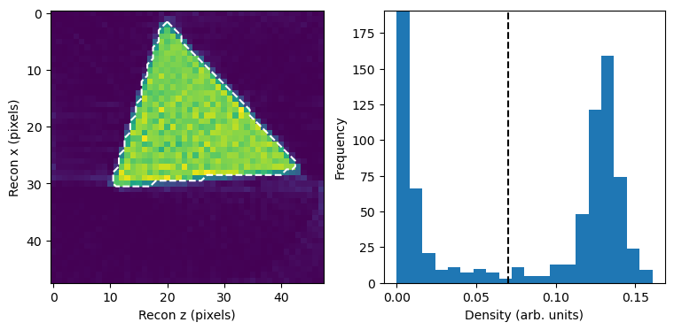
Basic plots of the reconstruction

For mono-phase samples, we want to see a distinct peak in the density-histogram. If not, something is probably wrong!

When we have a nice peak, we can pick a theshhold to distinguish between pixel inside and outside the sample.

# Pick a threshold value to determine what pixels to plot.
mask_threshold = 0.07

plt.figure(figsize = (9, 4))
dens = np.sum(coefficients, axis = -1)
mask = dens > mask_threshold

plt.subplot(1,2,1)
plt.imshow(dens)
plt.contour(mask[:,:,0], levels = [0.5], colors=[(1,1,1)],linestyles='dashed')
plt.xlabel('Recon z (pixels)'); plt.ylabel('Recon x (pixels)');

plt.subplot(1,2,2)
freq = plt.hist(dens.flatten(), bins = 20)[0]
plt.ylim(0, np.max(freq[5:])*1.2)
plt.plot([mask_threshold]*2, [0, np.max(freq[5:])*1.2], 'k--')
plt.xlabel('Density (arb. units)')
plt.ylabel('Frequency')
plt.savefig('../img/density_histogram.png')
plt.show()

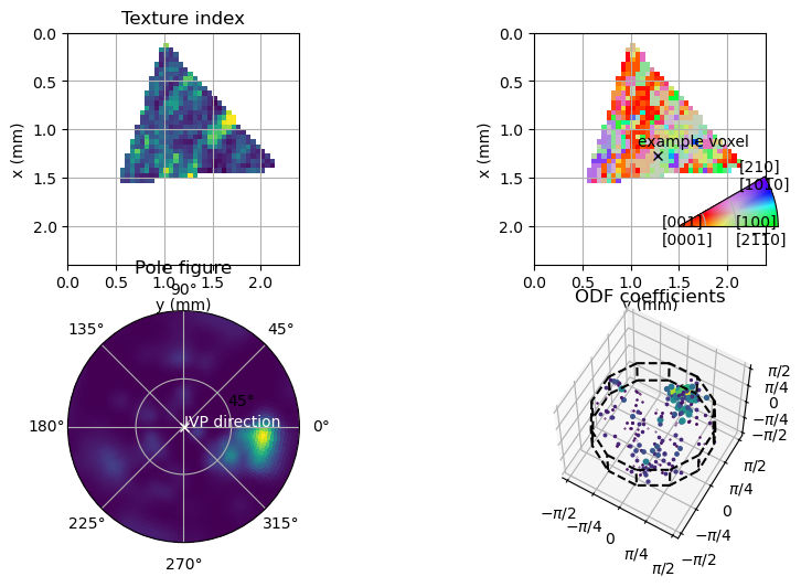
We plot a few basic quantities as tomograms as well as some twxture plots of a specific pixel. This sample consisit of some highly textures regions, where a single orientation dominates, as well as less texture regions where there are several differen crystal-orientations on the resolution of the experiments. The IVP-map is therefore only sensible in the textured regions.

# Pick a direction to compute the IPV map color
IVP_map_direction = np.array([0, 0, 1])
pole_figure_hkl = np.array([0, 0, 1])
coeffs_2d = coefficients[:,:,0,:]
example_voxel = (25, 25, 0)
stepsize = 0.05

imshow_opts = {'extent':(0, coeffs_2d.shape[0]*stepsize, coeffs_2d.shape[1]*stepsize, 0)}
pcolor_polar_opts = {'rasterized':True, 'vmin':0}

# Compute max direction IVP colormap
main_orientation_tomogram = odf_RBF.main_orientation(coefficients)
ipf_rgb_tomogram = odftomo.plot_tools.IPF_color(main_orientation_tomogram, IVP_map_direction, 'hexagonal')
ipf_rgb_tomogram[~mask, :] = 1


# Compute approximate texture index
J = np.sqrt(np.var(coefficients, axis = -1)) / np.mean(coefficients, axis = -1)
J[~mask] = np.nan

# Compute a pole-figure of a single voxel
voxel_coeffs = coefficients[example_voxel[0], example_voxel[1], example_voxel[2],:]
polefigure, theta_grid, phi_grid = odf_RBF.make_polefigure_map(voxel_coeffs,  B @ pole_figure_hkl)

/tmp/ipykernel_1904664/3289054818.py:18: RuntimeWarning: invalid value encountered in divide
  J = np.sqrt(np.var(coefficients, axis = -1)) / np.mean(coefficients, axis = -1)

# Build the plot
fig = plt.figure(figsize = (10, 6))

def tomogram_set_axes(ax):
    ax.set_xlabel('y (mm)')
    ax.set_ylabel('x (mm)')
    ax.grid()

# PLot IVP-map
ax = plt.subplot(2,2,2)
ax.imshow(ipf_rgb_tomogram[:, :, 0], **imshow_opts)
ax.plot((example_voxel[1]+0.5)*stepsize, (example_voxel[0]+0.5)*stepsize, 'kx')
ax.text((example_voxel[1]+0.5)*stepsize - 0.2, (example_voxel[0]+0.5)*stepsize - 0.1, 'example voxel', color = 'k')
tomogram_set_axes(ax)
ax = fig.add_subplot([0.72, 0.55, 0.15, 0.15], polar = True)
odftomo.plot_tools.make_color_legend(ax, 'hexagonal')

# Plot texture index
ax = plt.subplot(2,2,1)
img = ax.imshow(J[:, :, 0], **imshow_opts, vmax = 8)
tomogram_set_axes(ax)
ax.set_title('Texture index')

# PLot pole figure
ax = plt.subplot(2,2,3, polar=True)
img = ax.pcolormesh(phi_grid, np.tan(theta_grid/2), polefigure, **pcolor_polar_opts)
ax.set_yticks([np.tan(ii*np.pi/8) for ii in range(1,2)])
ax.set_yticklabels(['45°'])
ax.yaxis.label.set_color('w')
ax.set_title('Pole figure')

IVP_map_theta = np.arctan2(np.sqrt(IVP_map_direction[0]**2+IVP_map_direction[1]**2), IVP_map_direction[2])
IVP_map_phi = np.arctan2(IVP_map_direction[1], IVP_map_direction[0])
ax.plot(IVP_map_phi, np.tan(IVP_map_theta/2), 'wx')
ax.text(IVP_map_phi+0.3, np.tan(IVP_map_theta/2), 'IVP direction',color = 'w')

# PLot ODF modes in Rodriguez
ax = plt.subplot(2,2,4, projection='3d')
voxel_coeffs = coefficients[example_voxel[0], example_voxel[1], example_voxel[2],:]
odftomo.plot_tools.plot_orientation_coeffs(voxel_coeffs, odf_RBF.grid, ax, point_group_string='hexagonal')
ax.view_init(elev = 60)
ax.set_title('ODF coefficients')

fig.tight_layout()
fig.show()

/tmp/ipykernel_1904664/2671846072.py:44: UserWarning: This figure includes Axes that are not compatible with tight_layout, so results might be incorrect.
  fig.tight_layout()
/tmp/ipykernel_1904664/2671846072.py:44: UserWarning: Tight layout not applied. The left and right margins cannot be made large enough to accommodate all Axes decorations.
  fig.tight_layout()

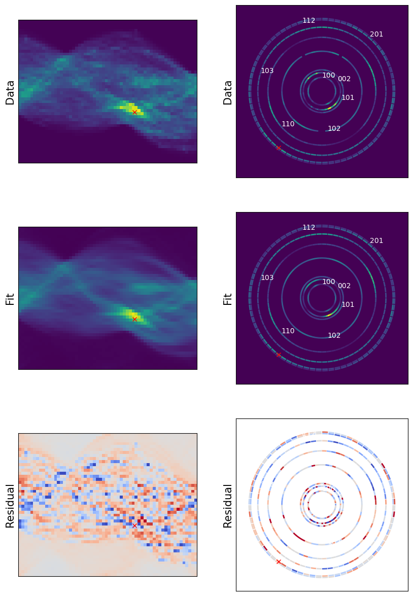
Evaluate quality of fit

To evaluate the quality of the reconstruction, we can look at the residual of the fit to the data. First, we run the forward model on the reconstruction to find the projected intensitites.

projected_intensities = model_RBF.forward(coefficients)

Because the data is 4-dimensional, it can be a bit tricky to visualize the fit. Here are two suggestions of how to do it:

1. Pick one scattering channel (a hkl and and azimth) and plot the 2D sinograms for that channel.

2. Pick a single sample position and orientation and plot the diffraction pattern at that point.

Neither plot nor the combination of the two contains all the relevant data, but both can be used to identify certain problems in the reconstructions, such as too low resolution and erroneous data-corrections like wrong form-factors, missing transmission correction or a faulty geometry.

hkl_index = 6
azim_index = 10
rotation_index = 38
position_index = 30


plt.figure(figsize = (10,15))
vmax = 1.0*np.max(data_array[:,:,0,azim_index,hkl_index])

### Plot single-channel sinograms
plt.subplot(3,2,1)
plt.imshow(data_array[:, :, 0, azim_index, hkl_index].T, vmax = vmax, vmin = 0)
plt.ylabel('Data', fontsize = 15)
plt.xticks([]); plt.yticks([])
plt.plot(rotation_index + 0.5, position_index+0.5, 'rx')

plt.subplot(3,2,3)
plt.imshow(projected_intensities[:, :, 0, azim_index, hkl_index].T, vmax = vmax, vmin = 0)
plt.ylabel('Fit', fontsize = 15)
plt.xticks([]); plt.yticks([])
plt.plot(rotation_index + 0.5, position_index+0.5, 'rx')

plt.subplot(3,2,5)
plt.imshow(projected_intensities[:, :, 0, azim_index, hkl_index].T-data_array[:, :, 0, azim_index, hkl_index].T,
           cmap = 'coolwarm', vmin = -0.1*vmax, vmax = 0.1*vmax)
plt.ylabel('Residual', fontsize = 15)
plt.xticks([]); plt.yticks([])
plt.plot(rotation_index + 0.5, position_index+0.5, 'rx')

### Plot single diffraction patterns
# Calculate the twotheta angles. This only works when making some assumption about the geometry.
twothetas_list = np.arcsin(np.abs(coordinates[0,0,0,0,:,1]))*2
azim_values = full_geom.detector_angles[azim_index]

def set_diffraction_pattern_axes(ax):
    for ii, (twotheta, hkl) in enumerate(zip(twothetas_list, hkl_list)):
        ax.text(np.tan(twotheta)*np.sin(ii*1.0), np.tan(twotheta)*np.cos(ii*1.0), f'{hkl[0]}{hkl[1]}{hkl[2]}' , color = 'w')
    ax.set_xlim(-0.11, 0.11)
    ax.set_ylim(-0.11, 0.11)
    ax.set_xticks([])
    ax.set_yticks([])
    ax.plot(np.cos(azim_values) * np.tan(twothetas_list[hkl_index]), np.sin(azim_values) * np.tan(twothetas_list[hkl_index]), 'rx')

ax = plt.subplot(3,2,2)
scatt_data = data_array[rotation_index, position_index, 0, :, :]
odftomo.plot_tools.plot_simulated_diffraction_pattern(full_geom, twothetas_list, scatt_data=scatt_data, ax = ax)
set_diffraction_pattern_axes(ax)
ax.set_ylabel('Data', fontsize = 15)

ax = plt.subplot(3,2,4)
scatt_data = projected_intensities[rotation_index, position_index, 0, :, :]
odftomo.plot_tools.plot_simulated_diffraction_pattern(full_geom, twothetas_list, scatt_data=scatt_data, ax = ax)
set_diffraction_pattern_axes(ax)
ax.set_ylabel('Fit', fontsize = 15)

ax = plt.subplot(3,2,6)
scatt_data = data_array[rotation_index, position_index, 0, :, :] - projected_intensities[rotation_index, position_index, 0, :, :]
scatt_data[weigth_array[rotation_index, position_index, 0, :, :] < 0.5] = 0.0
vmax = np.max(np.abs(scatt_data))*0.2
odftomo.plot_tools.plot_simulated_diffraction_pattern(full_geom, twothetas_list, scatt_data=scatt_data, ax = ax,
                                                    cmap = mpl.cm.get_cmap('coolwarm'), maxdata = vmax, mindata = -vmax, bg_color = [1, 1, 1])
set_diffraction_pattern_axes(ax)
ax.set_ylabel('Residual', fontsize = 15)

plt.show()

/tmp/ipykernel_1904664/3546156372.py:61: MatplotlibDeprecationWarning: The get_cmap function was deprecated in Matplotlib 3.7 and will be removed in 3.11. Use ``matplotlib.colormaps[name]`` or ``matplotlib.colormaps.get_cmap()`` or ``pyplot.get_cmap()`` instead.
  cmap = mpl.cm.get_cmap('coolwarm'), maxdata = vmax, mindata = -vmax, bg_color = [1, 1, 1])

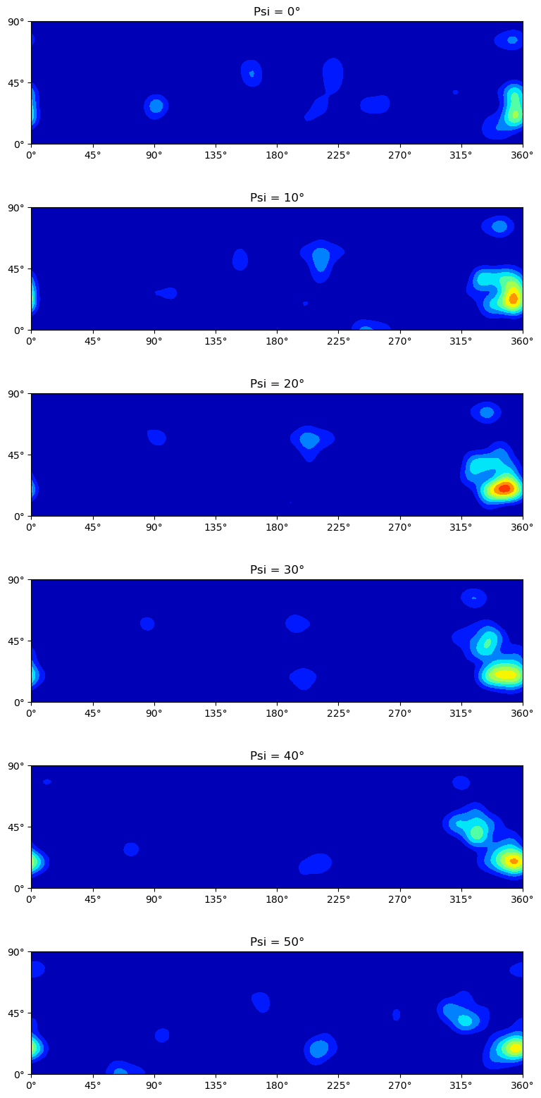
Euler sections

# Euler-sections of single-pixel texture
Psi = np.linspace(0, 2*np.pi/6, 6, endpoint=False)
Theta = np.linspace(0, np.pi/2, 90//2+1)
Phi = np.linspace(0, 2*np.pi, 360//2+1)

ODF_map, (Psi_map, Theta_map, Phi_map) = RBF_mapper(voxel_coeffs,
                                                    odf_RBF,
                                                    euler_angles_tuple=(Psi, Theta, Phi),
                                                    strategy='spharm')
ODF_map = ODF_map/np.sum(voxel_coeffs)

plt.figure(figsize = (9, 20))
for ii in range(6):
    ax= plt.subplot(6,1,ii+1)
    plt.contourf(np.clip(ODF_map[ii,:,:], 0, np.inf), extent = (0, Phi[-1]*180/np.pi, Theta[-1]*180/np.pi, 0),
                 levels=np.linspace(0, 30, 11), cmap='jet')
    plt.title(f'Psi = {Psi_map[0, 0, ii]*180/np.pi:.0f}°')
    ax.set_aspect("equal")
    ticks = np.arange(0, Theta[-1]*180/np.pi+45, 45); labels = [f'{t:.0f}°' for t in ticks]
    plt.yticks(ticks, labels=labels)
    ticks = np.arange(0, Phi[-1]*180/np.pi+45, 45); labels = [f'{t:.0f}°' for t in ticks]
    plt.xticks(ticks, labels=labels)
plt.show()

/das/home/carlse_m/grids_in_so3/odftt/spharm/RBF_mapper.py:81: UserWarning: Gimbal lock detected. Setting third angle to zero since it is not possible to uniquely determine all angles.
  transform = RBF_to_GSH(RBF_coeffs, odf_RBF, ell_max)
100%|██████████| 33/33 [00:28<00:00,  1.17it/s]