Demonstration using grid based functions

This notebook demonstrates the reconstruction workflow for a single-slice reconstruction using grid-based Gaussian basis functions. The method is documented in https://arxiv.org/abs/2407.11022 and the experiment is described in https://doi.org/10.1107/S160057672400400X

1. Imports

import numpy as np
from tqdm import tqdm
from odftomo.io import load_series, slice_geometry
from odftomo.texture import grids, point_groups, odfs
from odftomo.tomography_models import FromArrayModel
from odftomo.crystallography import cubic
from odftomo.optimization import FISTA
from odftomo.spharm.RBF_mapper import RBF_mapper

import matplotlib as mpl
import matplotlib.pyplot as plt
import matplotlib.gridspec as gridspec
from odftomo import plot_tools

import logging
logger = logging.getLogger()
logger.setLevel(logging.ERROR)

INFO:Setting the number of threads to 4. If your physical cores are fewer than this number, you may want to use numba.set_num_threads(n), and os.environ["OPENBLAS_NUM_THREADS"] = f"{n}" to set the number of threads to the number of physical cores n.
INFO:Setting numba log level to WARNING.

2. Loading data

We use the mumott data loader to ensure compatibility. Because mumott does for now not have explicit support for files with multiple q-bins, this involves separately loading a file for each q-bin. odftomo.io.load_series wraps this behaviour and outputs the arrays we need:

1. data_array is a 5D numpy array containing the azimtuthally regrouped data ordered like: 0 sample rotation, 1 first raster scan index, 2 second raster scan index ( for a single-slice experiment this should have length 1), 3 detector azimuthal angle, 4 bragg peak number.

2. weigth_array used to weight the residual for optimization. Mainly used to mask out bad data. Same shape as data_array.

3. coordinates unit vectors of the q-space direction in sample-fixed coordinates probed by each data point. The shape of the array shoudl match data_array but with one-length dimensions for the two raster-scan indexes: Shape is 0 sample rotation, 1 and 2 are 1-length dimensions corresponding the the sample-scannign directions used to make broadcasting easier, the 3 index is the detector azimuth, 4 bragg peak number and 5 is the vector xyz index.

4. geometry mumott geometry object used to initialize the projector object later which is used to calculate radon transforms. For a description of this object see mumott.org.

The data used for this demonstration is publically available at: https://zenodo.org/records/10889439

wget https://zenodo.org/records/10889439/files/gamma_111.h5 https://zenodo.org/records/10889439/files/gamma_200.h5 https://zenodo.org/records/10889439/files/gamma_220.h5

hkl_list = [(1, 1, 1),
            (2, 0, 0),
            (2, 2, 0),]
files = [f'gamma_{h[0]}{h[1]}{h[2]}.h5' for h in hkl_list]
data_array, weigth_array, coordinates, full_geom = load_series(files)

/das/home/carlse_m/mumott_dev_version/mumott/mumott/data_handling/data_container.py:227: DeprecationWarning: Entry name rotations is deprecated. Use inner_angle instead.
  _deprecated_key_warning('rotations')
/das/home/carlse_m/mumott_dev_version/mumott/mumott/data_handling/data_container.py:236: DeprecationWarning: Entry name tilts is deprecated. Use outer_angle instead.
  _deprecated_key_warning('tilts')
/das/home/carlse_m/mumott_dev_version/mumott/mumott/data_handling/data_container.py:268: DeprecationWarning: Entry name offset_j is deprecated. Use j_offset instead.
  _deprecated_key_warning('offset_j')
/das/home/carlse_m/mumott_dev_version/mumott/mumott/data_handling/data_container.py:278: DeprecationWarning: Entry name offset_k is deprecated. Use k_offset instead.
  _deprecated_key_warning('offset_k')
/das/home/carlse_m/grids_in_so3/odftt/io/mumott_fileformat_loader.py:26: RuntimeWarning: invalid value encountered in divide
  data_arrays.append(np.array(data_container.data / data_container.diode[:, :, :, np.newaxis]))

For this demonstration to run quickly on slow hardware, we reconstruct only a 2D slice. This block can be omitted if you want to do a 3D reconstruction, but it will be slow! We achieve a 2D geometry by removing all measurements with tilt-angle not equal to 0 and to select only a single 1D slice of the 2D raster scans.

# Include only projecitons with zero tilt.
data_array = data_array[:50, ...]
weigth_array = weigth_array[:50, ...]
coordinates = coordinates[:50, ...]
geom = slice_geometry(full_geom, slice(50))

# Crop out a single 1D slice of the 2D raster scans
data_slice = data_array[:,:,25:26,:,:]
weigth_slice = weigth_array[:,:,25:26,:,:]

# Make a new mumott geometry object corresponding to the 2D geometry
from mumott.core.geometry import Geometry, GeometryTuple
geom_slice = Geometry()
for gt in geom:
    gt_new = GeometryTuple(rotation = gt.rotation, k_offset = 0.0, j_offset = 0)
    geom_slice.append(gt_new)
geom_slice.volume_shape = np.array([60, 1, 60])
geom_slice.projection_shape = np.array([54, 1])
geom_slice.p_direction_0 = geom.p_direction_0
geom_slice.j_direction_0 = geom.j_direction_0
geom_slice.k_direction_0 = geom.k_direction_0
geom_slice.detector_direction_origin = geom.detector_direction_origin
geom_slice.detector_direction_positive_90 = geom.detector_direction_positive_90
geom_slice.detector_angles = geom.detector_angles
geom_slice.full_circle_covered = geom.full_circle_covered

If we assume that the dataset is well sampled over all crystallographic directions, we don’t have to model the scattering form-factors. We can simply normalize this out of the data. We always normalize the formfactors (and other |q|-dependent quantities) out of the data to not bias the reconstruciton to the high-intensity reflections.

data_array[np.isnan(data_array) ] = 0
data_array[np.isinf(data_array) ] = 0
solidangle_factor = np.abs(np.cos(geom_slice.detector_angles))[np.newaxis,np.newaxis,np.newaxis,:,np.newaxis] * np.ones(data_array.shape)
intensity_scaling_factors = np.mean(data_array * solidangle_factor, axis = (0,1,2,3)) / np.mean(solidangle_factor, axis = (0,1,2,3))
intensity_scaling_factors = intensity_scaling_factors/intensity_scaling_factors[0]
data_slice = data_slice / intensity_scaling_factors[np.newaxis, np.newaxis, np.newaxis, np.newaxis, :]

3. Define reconstruction model

In this demonstration we use a basis of gaussian radially symmetric functions placed on a grid-of-orientations. The model is deifned by a function an orientation grid, a crystal symmetry point group, and a kernel width parameter. The grid is expected to match the symmetry group.

grid_resolution_parameter determines the number of grid points and kernel_sigma determines the width of each basis function. The two have to be chosen to match.

The odf object abstractly represents a model for ODFs and allows the probablity density function, pole-figures and inverse pole-figures of each basis function to be computed but does not keep track of the coefficients.

grid_resolution_parameter = 15 # (the heuristic way I do the griding tends to perform better with odd numbers)
grid = grids.hopf_grid(grid_resolution_parameter, point_groups.cubic)

odf = odfs.GaussianRBF(grid, point_groups.cubic)
print(f'Kernel sigma = {odf.sigma*180/np.pi:.1f}°')
print(f'The grid contains {odf.n_modes} orientations.')

Kernel sigma = 5.0°
The grid contains 612 orientations.

fig = plt.figure(figsize = (9, 9))

ax = plt.subplot(2,2,1, projection = '3d')
plot_tools.plot_asym_zone_outline(ax, 'cubic')
plot_tools.plot_asym_zone_outline(ax, 'none')
for s in point_groups.cubic:
    plt.plot(*s.as_rotvec(), 'x', markeredgewidth=3, markersize=10)
ax.set_title(r'Point group rotations $s_i\in S$')

ax = plt.subplot(2,2,2, projection = '3d')
plot_tools.plot_asym_zone_outline(ax, 'cubic')
plot_tools.plot_asym_zone_outline(ax, 'none')
rotvecs = odf.grid.as_rotvec()
ax.scatter(rotvecs[:,0], rotvecs[:,1], rotvecs[:,2], s = 1)
ax.set_title(r'Grid orientations $g_m$')

ax = plt.subplot(2,2,3, projection = '3d')
plot_tools.plot_asym_zone_outline(ax, 'cubic')
plot_tools.plot_asym_zone_outline(ax, 'none')
rotvecs = (odf.grid*point_groups.cubic[3]).as_rotvec()
ax.scatter(rotvecs[:,0], rotvecs[:,1], rotvecs[:,2], s = 1, c = 'C3')
ax.set_title(r'Shifted grid orientations $g_ms_3$')

ax = plt.subplot(2,2,4, projection = '3d')
plot_tools.plot_asym_zone_outline(ax, 'cubic')
plot_tools.plot_asym_zone_outline(ax, 'none')
for s_index, s in enumerate(point_groups.cubic):
    rotvecs = (odf.grid*point_groups.cubic[s_index]).as_rotvec()
    ax.scatter(rotvecs[:,0], rotvecs[:,1], rotvecs[:,2], s = 1)
ax.set_title(r'Shifted grid orientations $g_ms_i$')
plt.savefig('../img/cubic_orientation_grid.png')
fig.show()

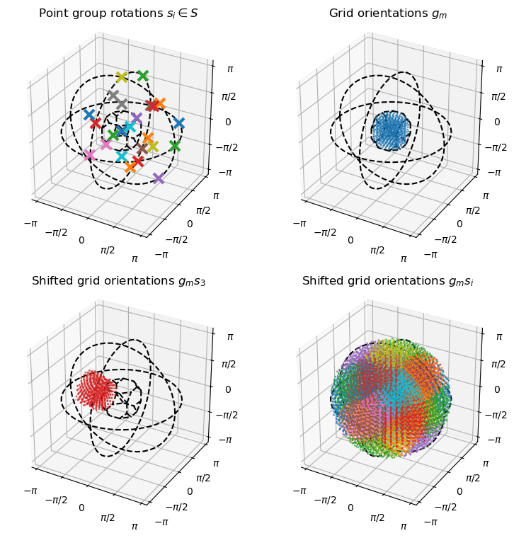
The orientation grid fills one assumetric unit of rotation space (b), such that if the grid is shifted by all the point group symmetries(a), it fills out all of orientation space without overlapping itself(d).

We plot a pole figure of a single basis mode. Then we compute a set of orientations that approximately fall on a fiber texture and plot this in 3 different ways.

# Find modes close to a fiber
fiber_realspace_orientation = np.array([1, 2, 3])
fiber_latticespace_orientation = np.array([1, 1, 1])
fiber_realspace_orientation = fiber_realspace_orientation / np.linalg.norm(fiber_realspace_orientation)
fiber_latticespace_orientation = fiber_latticespace_orientation / np.linalg.norm(fiber_latticespace_orientation)
modes_on_fiber = np.zeros(odf.n_modes, dtype = bool)
for gs in odf.point_group:
    h = (odf.grid*gs).apply(fiber_latticespace_orientation)
    modes_on_fiber += np.arccos(h @ fiber_realspace_orientation) < 0.15
print(f'There are {np.sum(modes_on_fiber)} modes on the fiber')
fibre_coefficients = np.zeros(odf.n_modes)
fibre_coefficients[modes_on_fiber] = 1

There are 28 modes on the fiber

fig = plt.figure(figsize = (9, 7))

# Pole figure of single basisfunction
ax = plt.subplot(2,2,1, polar=True)
voxel_coefficients = np.zeros(odf.n_modes)
voxel_coefficients[7] = 1
polefigure, theta_grid, phi_grid = odf.make_polefigure_map(voxel_coefficients, np.array([1,0,0]))
img = ax.pcolormesh(phi_grid, np.tan(theta_grid/2), polefigure, rasterized=True)
plt.colorbar(img)
plt.title('Single basisfunction PF')
ax.set_yticks(np.tan(np.array([0, np.pi/4, np.pi/2])/2), labels = ['0°', '45°', '90°'], color = 'w')

# Pole figure of fibre
ax = plt.subplot(2,2,2, polar=True)
polefigure, theta_grid, phi_grid = odf.make_polefigure_map(fibre_coefficients, np.array([1,0,0]))
img = ax.pcolormesh(phi_grid, np.tan(theta_grid/2), polefigure, rasterized=True)
plt.colorbar(img)
plt.title('Fibre texture (100) PF')
ax.set_yticks(np.tan(np.array([0, np.pi/4, np.pi/2])/2), labels = ['0°', '45°', '90°'], color = 'w')

# Inverse pole figure of fibre
ax = plt.subplot(2,2,3, polar=True)
inverse_polefigure, theta_grid, phi_grid = odf.make_inverse_polefigure_map(
    fibre_coefficients, fiber_realspace_orientation, resolution_in_degrees=1.0)

# Crop inverse pole figure to asymmetric zone
inverse_polefigure[phi_grid>45*np.pi/180] = np.nan # Line from [001] to [111]
inverse_polefigure[phi_grid<0] = np.nan # Line from [001] to [101]
grid_x = np.cos(phi_grid)*np.sin(theta_grid)
grid_z = np.cos(theta_grid)
inverse_polefigure[grid_x > grid_z] = np.nan

img = ax.pcolormesh(phi_grid, np.tan(theta_grid/2), inverse_polefigure, rasterized=True)
ax.set_yticks([np.tan(ii*np.pi/8) for ii in range(1,2)])
ax.set_yticklabels(['45°'])
ax.yaxis.label.set_color('w')
plt.xlim(0, 46*np.pi/180)
plt.ylim(0, np.tan(59*np.pi/180/2))
plt.axis('off')
plt.colorbar(img)
plt.title('Fibre texture IPF')
plot_tools.polefigure.plot_cubic_asym_outline(ax, color = 'k')

# FIbre texture plotted in rotvector representation
ax = fig.add_subplot(2, 2, 4, projection='3d')

for modenumber in np.arange(odf.n_modes)[modes_on_fiber]:
    rotvec = odf.grid[modenumber].as_rotvec()
    ax.plot(*rotvec, '.k')

plot_tools.set_rotvec_ax(ax, np.pi/4)
plot_tools.plot_asym_zone_outline(ax, 'cubic')
plt.savefig('../img/RBF_overview.png')
plt.show()

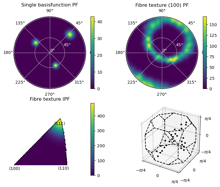
If the fibre texture looks choppy, you have picked kernel_sigma too small!

Define the lattice matrix used to convert Miller indicies into \(\mathbf{h}\)-vectors and initialize the forward model of the reconstruction problem. In the cubic system, this is not strictly necessary, but we do it anyways to build good habits.

A, B = cubic()
h_vectors = [B @ hkl for hkl in hkl_list]

Now we need to define the full forward model which is a composition of a pole-figure transform and a Radon transform:

The pole figure transform is performed by a list of pre-computed arrays containging the scattering intensities of the individual texture basis function modes.

basis_function_arrays = odf.compute_polefigure_matrices_parallel(coordinates, h_vectors, num_processes=4)
model = FromArrayModel(basis_function_arrays, geom_slice)

Starting parallel computation of polefiugres.

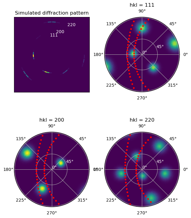
To show the meaning of these matrices, we plot how one basisfunction contibutes to the intensity measured at a specific orientation of the sample.

The basis_function_arrays is a list over sample orientations where each element is an unraveled matrix that maps each basis function to the detector channels \((\eta, hk\ell)\). It is unraveled like this to make it easy to switch between dense and sparse matrices (or anything else that overloads the matmul operator).

The values can be thought of as point-samples of the basis-function pole-figures, sampled on the points where the Ewald’s sphere intersects the shells \(|q| = \frac{4\pi}{\lambda}\sin(2\theta_{hkl\ell}/2)\).

# Compute polefures three measured rings
rotation_index = 35
basis_fun_number = 111
voxel_coefficients = np.zeros(odf.n_modes)
voxel_coefficients[basis_fun_number] = 1
polefigures = []
for hkl in hkl_list[:3]:
    polefigure, theta_grid, phi_grid = odf.make_polefigure_map(voxel_coefficients, np.array(hkl))
    polefigures.append(polefigure)

# This line only works when making some assumption about the geometry.
twothetas_list = np.arcsin(np.abs(coordinates[0,0,0,0,:,2]))*2
scatt_data = np.zeros(model.basisfunctions[0].shape[1])

for modenumber in np.arange(odf.n_modes)[basis_fun_number:basis_fun_number+1]:
    scatt_data+=model.basisfunctions[rotation_index][modenumber, :]
scatt_data = scatt_data.reshape(model.channels_shape)

fig = plt.figure(figsize = (7, 9))

ax = plt.subplot(2,2,1)
plot_tools.plot_simulated_diffraction_pattern(geom_slice, twothetas_list, scatt_data=scatt_data, ax = ax)

for ii, (twotheta, hkl) in enumerate(zip(twothetas_list, hkl_list)):
    plt.text(np.tan(twotheta)*np.sin(ii*0.3-0.1), np.tan(twotheta)*np.cos(ii*0.3-0.1),
             f'{hkl[0]}{hkl[1]}{hkl[2]}' , color='w')

ax.set_title('Simulated diffraction pattern')
ax.set_xlim(-0.7, 0.7); ax.set_ylim(-0.7, 0.7)
ax.set_xticks([]); ax.set_yticks([])

for hkl_index, hkl in enumerate(hkl_list[:3]):

    ax = plt.subplot(2,2,hkl_index+2, polar=True)
    img = ax.pcolormesh(phi_grid, np.tan(theta_grid/2), np.sqrt(polefigures[hkl_index]),
                        vmin=0, vmax=np.sqrt(np.max(polefigures)), rasterized=True)
    plt.title(f'hkl = {hkl[0]}{hkl[1]}{hkl[2]}')
    coords_vectors = coordinates[rotation_index, 0, 0, :, hkl_index, :]
    whereflip = coords_vectors[:,2] < 0
    coords_vectors[whereflip] = -coords_vectors[whereflip]
    thetas = np.arccos(coords_vectors[:, 2])
    phis = np.arctan2(coords_vectors[:, 1], coords_vectors[:, 0])
    for azim_index, (phi, theta) in enumerate(zip(phis, thetas)):
        ax.plot(phi, np.tan(theta/2), '.r')
        ax.set_yticks(np.tan(np.array([0, np.pi/4, np.pi/2])/2), labels = ['0°', '45°', '90°'], color = 'w')
plt.show()

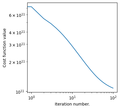
4. Run actual reconstruction

With the model defined, the reconstruction is a simple least-sqares problem:

optimizer = FISTA(model, data_slice, weights = weigth_slice, maxiter = 100)
x, convergence_curve = optimizer.optimize()

fig = plt.figure(figsize = (4,4))
plt.loglog(convergence_curve)
plt.xlabel('Iteration number.')
plt.ylabel('Cost function value')
plt.show()

Estimating largest safe step size

Matrix norm estimate = 2.50E+08:  60%|██████    | 6/10 [00:23<00:15,  3.84s/it]
Loss = 1.08E+11: 100%|██████████| 100/100 [03:47<00:00,  2.28s/it]

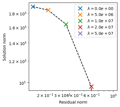
The quality of the reconstruction can sometimes benefit from L1-regularization. Here we run a sweep of the regularization parameter to find a good value.

results_list = []
for reg_param in [0.0, 5e6, 1e7, 2e7, 5e7]:
    optimizer.regularization_weigth = reg_param
    x, convergence_curve = optimizer.optimize()
    results_list.append( {'reg_param':reg_param,'x': np.array(x), 'conv_curve':convergence_curve} )

Loss = 1.08E+11: 100%|██████████| 100/100 [00:29<00:00,  3.36it/s]
Loss = 2.44E+11: 100%|██████████| 100/100 [00:29<00:00,  3.42it/s]
Loss = 3.57E+11: 100%|██████████| 100/100 [00:33<00:00,  2.94it/s]
Loss = 5.36E+11: 100%|██████████| 100/100 [00:33<00:00,  3.03it/s]
Loss = 7.22E+11: 100%|██████████| 100/100 [00:28<00:00,  3.51it/s]

def get_res_norm(result):
    residual = model.forward(result['x']) - data_slice
    return np.sum(residual**2*weigth_slice) / np.sum(data_slice**2*weigth_slice)

res_norm = [get_res_norm(res) for res in results_list]
sol_norm = [np.sum(res['x']**2) for res in results_list]
reg_param = [res['reg_param'] for res in results_list]

fig = plt.figure(figsize = (4,4))
plt.loglog(res_norm, sol_norm, 'k--')
points = []

for ii in range(len(reg_param)):
    point, = plt.loglog(res_norm[ii], sol_norm[ii], 'x', markersize =10, markeredgewidth = 2)
    points.append(point)

plt.xlabel('Residual norm')
plt.ylabel('Solution norm')
plt.gca().legend(points, [fr'$\lambda = {p:.1e}$' for p in reg_param], )
plt.show()

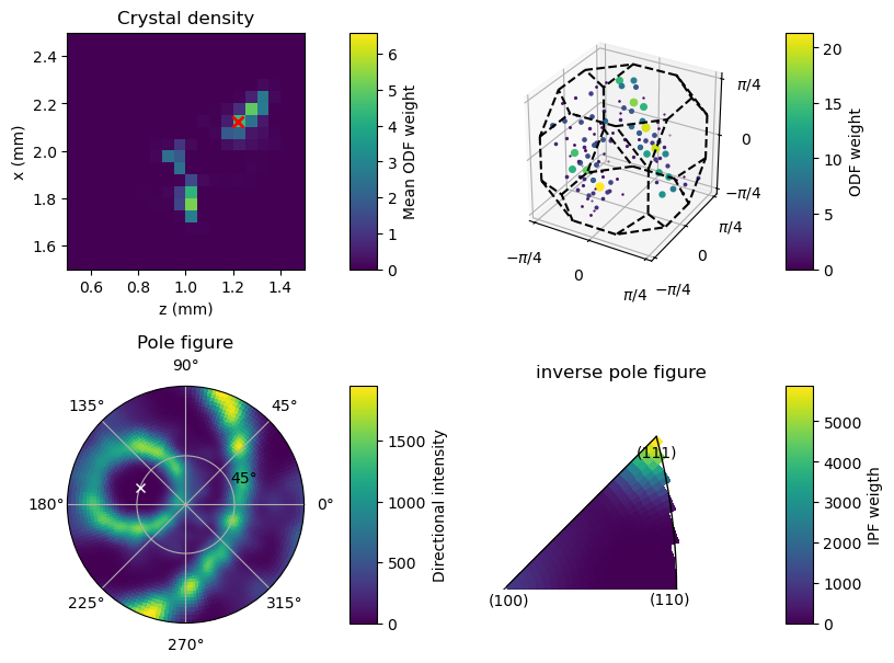
5. Basic plots of the reconstruction

There are other demonstration notebooks documenting the analysis of reconstructions. For this notebook, we just show do a basic plot showing a) the reconstructed density (which will only be non-zero in a few points where the reconstructed plane intersects the wire) and b) the ODF-modes of a specific voxel, c) a pole figure calculated from that same voxel and the corresponding inverse-pole-figure computed in the fibre-direction.

fig = plt.figure(figsize = (9, 7))
example_voxel = (18, 0, 24)
coeffs = results_list[1]['x'] # Select one from the list of regularized reconstructions
ipf_direction = (45*np.pi/180, 160*np.pi/180) # This is the direction in which the inverse pole-figure will be computed
ipf_xyz = [np.cos(ipf_direction[1])*np.sin(ipf_direction[0]),
           np.sin(ipf_direction[1])*np.sin(ipf_direction[0]),
           np.cos(ipf_direction[0]),]
pcolor_opts = {'vmin':0, 'rasterized':True}
imshow_opts = {'extent':(0,3,0,3)}#{'vmax':0.0005, 'extent':(0,3,0,3)}
plot_threshold = 0.05 # FOr the 3D ODF plot, remove low-weight modes to reduce clutter

gs = gridspec.GridSpec(3, 5, figure=fig, width_ratios=[1, 0.1, 0.2, 1, 0.1], height_ratios=[1, 0.2, 1,])
############# DENSITY SLICE #####################################
ax = fig.add_subplot(gs[0,0])
plt.imshow(np.sum(coeffs[:,example_voxel[1],:,:], axis = -1), **imshow_opts)
ax.set_xlim(0.5,1.5); ax.set_ylim(1.5,2.5)
plt.plot(example_voxel[2]*0.05+0.02, 3-example_voxel[0]*0.05+0.025, 'rx', markersize=7, markeredgewidth=2)
ax.set_xlabel('z (mm)')
ax.set_ylabel('x (mm)')
plt.title('Crystal density')
cax = fig.add_subplot(gs[0,1])
fig.colorbar(img, cax = cax, label = 'Mean ODF weight')

##############  SINGLE PIXEL POLEFIGURE ########################
ax = fig.add_subplot(gs[2,0], polar=True)
voxel_coeffs = coeffs[example_voxel[0], example_voxel[1], example_voxel[2],:]
polefigure, theta_grid, phi_grid = odf.make_polefigure_map(voxel_coeffs, np.array([1,1,0]))
img = ax.pcolormesh(phi_grid, np.tan(theta_grid/2), polefigure, **pcolor_opts)
ax.set_yticks([np.tan(ii*np.pi/8) for ii in range(1,2)])
ax.set_yticklabels(['45°'])
ax.yaxis.label.set_color('w')
plt.title('Pole figure')
plt.plot(ipf_direction[1], np.tan(ipf_direction[0]/2), 'wx')
cax = fig.add_subplot(gs[2,1])
fig.colorbar(img, cax = cax, label = 'Directional intensity')

##############  SINGLE PIXEL INVERSE POLEFIGURE ########################
ax = fig.add_subplot(gs[2,3], polar=True)
inverse_polefigure, theta_grid, phi_grid = odf.make_inverse_polefigure_map(voxel_coeffs, ipf_xyz)

# Crop inverse pole figure to asymmetric zone
inverse_polefigure[phi_grid>45*np.pi/180] = np.nan # Line from [001] to [111]
inverse_polefigure[phi_grid<0] = np.nan # Line from [001] to [101]
grid_x = np.cos(phi_grid)*np.sin(theta_grid)
grid_z = np.cos(theta_grid)
inverse_polefigure[grid_x > grid_z] = np.nan

img = ax.pcolormesh(phi_grid, np.tan(theta_grid/2), inverse_polefigure, **pcolor_opts)
ax.set_yticks([np.tan(ii*np.pi/8) for ii in range(1,2)])
ax.set_yticklabels(['45°'])
ax.yaxis.label.set_color('w')
plt.title('inverse pole figure')
plt.xlim(0, 46*np.pi/180)
plt.ylim(0, np.tan(59*np.pi/180/2))
plt.axis('off')
plot_tools.polefigure.plot_cubic_asym_outline(ax)
cax = fig.add_subplot(gs[2,4])
fig.colorbar(img, cax = cax, label = 'IPF weigth')

#################### PLOT ODF WEIGHTS IN 3D VIEW  ######################
ax = fig.add_subplot(gs[0,3],projection='3d')
max_coeff = np.max(voxel_coeffs)
plot_tools.plot_orientation_coeffs(voxel_coeffs, odf.grid, ax, point_group_string='cubic')

cax = fig.add_subplot(gs[0,4])
norm = mpl.colors.Normalize(vmin=0, vmax=max_coeff, clip=False)
fig.colorbar(mpl.cm.ScalarMappable(norm=norm, cmap=mpl.colormaps['viridis']) ,cax = cax, label = 'ODF weight')
plt.show()

/tmp/ipykernel_2149750/1938821913.py:22: UserWarning: Adding colorbar to a different Figure <Figure size 700x900 with 4 Axes> than <Figure size 900x700 with 2 Axes> which fig.colorbar is called on.
  fig.colorbar(img, cax = cax, label = 'Mean ODF weight')

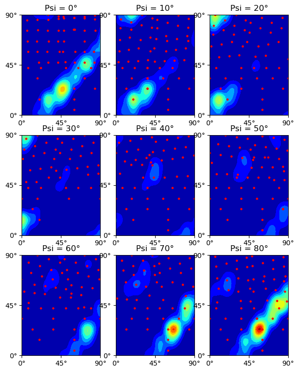
For closer comparison with the GSH reconstructions, we calculate Euler angle sections of a single voxel.

# Euler-sections of single-pixel texture
Psi = np.linspace(0, np.pi/2, 9, endpoint=False)
Psi_step = np.abs(Psi[1] - Psi[0])
Theta = np.linspace(0, np.pi/2, 51, endpoint=False)
Phi = np.linspace(0, np.pi/2, 51, endpoint=False)

ODF_map, (Psi_map, Theta_map, Phi_map) = RBF_mapper(voxel_coeffs,
                                                    odf,
                                                    euler_angles_tuple = (Psi, Theta, Phi))
ODF_map = ODF_map/np.sum(voxel_coeffs)

plt.figure(figsize = (7, 9))
for ii in range(9):
    plt.subplot(3,3,ii+1)
    plt.contourf(ODF_map[ii,:,:], extent = (0, 90, 0, 90),
                 levels=np.linspace(0, 24, 13), cmap='jet')
    plt.title(f'Psi = {Psi_map[0, 0, ii]*180/np.pi:.0f}°')
    ticks = [0, 45, 90]; labels = ['0°', '45°', '90°']
    plt.xticks(ticks, labels=labels)
    plt.yticks(ticks, labels=labels)

    Psi_lim = [-Psi_step/2 + Psi[ii], +Psi_step/2 + Psi[ii]]
    for s in odf.point_group:
        g = odf.grid * s
        euler_angles = g.as_euler('zyz')
        euler_angles[:, 0] = ((euler_angles[:, 0] + np.pi) % (2*np.pi) ) - np.pi
        in_slice_inxd = np.logical_and(euler_angles[:,0] >= Psi_lim[0], euler_angles[:,0] < Psi_lim[1])
        plt.scatter(euler_angles[in_slice_inxd, 2]*180/np.pi,
                    euler_angles[in_slice_inxd, 1]*180/np.pi,
                    color='r', s=5.0)
    plt.xlim(0, 90); plt.ylim(0, 90)
plt.show()